Design Red Off Systemc Using Dynamic Processes

Simulation Manual

OMNeT++ version 5.6.1

http://omnetpp.org

Chapters

1 Introduction
2 Overview
3 The NED Language
4 Simple Modules
5 Messages and Packets
6 Message Definitions
7 The Simulation Library
8 Graphics and Visualization
9 Building Simulation Programs
10 Configuring Simulations
11 Running Simulations
12 Result Recording and Analysis
13 Eventlog
14 Documenting NED and Messages
15 Testing
16 Parallel Distributed Simulation
17 Customizing and Extending OMNeT++
18 Embedding the Simulation Kernel
19 Appendix A: NED Reference
20 Appendix B: NED Language Grammar
21 Appendix C: NED XML Binding
22 Appendix D: NED Functions
23 Appendix E: Message Definitions Grammar
24 Appendix F: Display String Tags
25 Appendix G: Figure Definitions
26 Appendix H: Configuration Options
27 Appendix I: Result File Formats
28 Appendix J: Eventlog File Format

  1 Introduction
    1.1 What Is OMNeT++?
    1.2 Organization of This Manual

  2 Overview
    2.1 Modeling Concepts
2.1.1 Hierarchical Modules
2.1.2 Module Types
2.1.3 Messages, Gates, Links
2.1.4 Modeling of Packet Transmissions
2.1.5 Parameters
2.1.6 Topology Description Method
    2.2 Programming the Algorithms
    2.3 Using OMNeT++
2.3.1 Building and Running Simulations
2.3.2 What Is in the Distribution

  3 The NED Language
    3.1 NED Overview
    3.2 NED Quickstart
3.2.1 The Network
3.2.2 Introducing a Channel
3.2.3 The App, Routing, and Queue Simple Modules
3.2.4 The Node Compound Module
3.2.5 Putting It Together
    3.3 Simple Modules
    3.4 Compound Modules
    3.5 Channels
    3.6 Parameters
3.6.1 Assigning a Value
3.6.2 Expressions
3.6.3 volatile
3.6.4 Units
3.6.5 XML Parameters
    3.7 Gates
    3.8 Submodules
    3.9 Connections
3.9.1 Channel Specification
3.9.2 Reconnecting Gates
3.9.3 Channel Names
    3.10 Multiple Connections
3.10.1 Examples
3.10.2 Connection Patterns
    3.11 Parametric Submodule and Connection Types
3.11.1 Parametric Submodule Types
3.11.2 Conditional Parametric Submodules
3.11.3 Parametric Connection Types
    3.12 Metadata Annotations (Properties)
3.12.1 Property Indices
3.12.2 Data Model
3.12.3 Overriding and Extending Property Values
    3.13 Inheritance
    3.14 Packages
3.14.1 Overview
3.14.2 Name Resolution, Imports
3.14.3 Name Resolution With "like"
3.14.4 The Default Package

  4 Simple Modules
    4.1 Simulation Concepts
4.1.1 Discrete Event Simulation
4.1.2 The Event Loop
4.1.3 Events and Event Execution Order in OMNeT++
4.1.4 Simulation Time
4.1.5 FES Implementation
    4.2 Components, Simple Modules, Channels
    4.3 Defining Simple Module Types
4.3.1 Overview
4.3.2 Constructor
4.3.3 Initialization and Finalization
    4.4 Adding Functionality to cSimpleModule
4.4.1 handleMessage()
4.4.2 activity()
4.4.3 How to Avoid Global Variables
4.4.4 Reusing Module Code via Subclassing
    4.5 Accessing Module Parameters
4.5.1 Volatile and Non-Volatile Parameters
4.5.2 Changing a Parameter's Value
4.5.3 Further cPar Methods
4.5.4 Emulating Parameter Arrays
4.5.5 handleParameterChange()
    4.6 Accessing Gates and Connections
4.6.1 Gate Objects
4.6.2 Connections
4.6.3 The Connection's Channel
    4.7 Sending and Receiving Messages
4.7.1 Self-Messages
4.7.2 Sending Messages
4.7.3 Broadcasts and Retransmissions
4.7.4 Delayed Sending
4.7.5 Direct Message Sending
4.7.6 Packet Transmissions
4.7.7 Receiving Messages with activity()
    4.8 Channels
4.8.1 Overview
4.8.2 The Channel API
4.8.3 Channel Examples
    4.9 Stopping the Simulation
4.9.1 Normal Termination
4.9.2 Raising Errors
    4.10 Finite State Machines
4.10.1 Overview
    4.11 Navigating the Module Hierarchy
4.11.1 Module Vectors
4.11.2 Component IDs
4.11.3 Walking Up and Down the Module Hierarchy
4.11.4 Finding Modules by Path
4.11.5 Iterating over Submodules
4.11.6 Navigating Connections
    4.12 Direct Method Calls Between Modules
    4.13 Dynamic Module Creation
4.13.1 When To Use
4.13.2 Overview
4.13.3 Creating Modules
4.13.4 Deleting Modules
4.13.5 Module Deletion and finish()
4.13.6 Creating Connections
4.13.7 Removing Connections
    4.14 Signals
4.14.1 Design Considerations and Rationale
4.14.2 The Signals Mechanism
4.14.3 Listening to Model Changes
    4.15 Signal-Based Statistics Recording
4.15.1 Motivation
4.15.2 Declaring Statistics
4.15.3 Statistics Recording for Dynamically Registered Signals
4.15.4 Adding Result Filters and Recorders Programmatically
4.15.5 Emitting Signals
4.15.6 Writing Result Filters and Recorders

  5 Messages and Packets
    5.1 Overview
    5.2 The cMessage Class
5.2.1 Basic Usage
5.2.2 Duplicating Messages
5.2.3 Message IDs
5.2.4 Control Info
5.2.5 Information About the Last Arrival
5.2.6 Display String
    5.3 Self-Messages
5.3.1 Using a Message as Self-Message
5.3.2 Context Pointer
    5.4 The cPacket Class
5.4.1 Basic Usage
5.4.2 Identifying the Protocol
5.4.3 Information About the Last Transmission
5.4.4 Encapsulating Packets
5.4.5 Reference Counting
5.4.6 Encapsulating Several Packets
    5.5 Attaching Objects To a Message
5.5.1 Attaching Objects
5.5.2 Attaching Parameters

  6 Message Definitions
    6.1 Introduction
6.1.1 The First Message Class
    6.2 Messages and Packets
6.2.1 Defining Messages and Packets
6.2.2 Field Data Types
6.2.3 Initial Values
6.2.4 Enums
6.2.5 Fixed-Size Arrays
6.2.6 Variable-Size Arrays
6.2.7 Classes and Structs as Fields
6.2.8 Pointer Fields
6.2.9 Inheritance
6.2.10 Assignment of Inherited Fields
    6.3 Classes
    6.4 Structs
    6.5 Literal C++ Blocks
    6.6 Using C++ Types
6.6.1 Announcing Types to the Message Compiler
6.6.2 Making the C++ Declarations Available
6.6.3 Putting it Together
    6.7 Customizing the Generated Class
6.7.1 Customizing Method Names
6.7.2 Customizing the Class via Inheritance
6.7.3 Abstract Fields
    6.8 Using Standard Container Classes for Fields
6.8.1 Typedefs
6.8.2 Abstract Fields
    6.9 Namespaces
6.9.1 Declaring a Namespace
6.9.2 C++ Blocks and Namespace
6.9.3 Type Announcements and Namespace
    6.10 Descriptor Classes
    6.11 Summary

  7 The Simulation Library
    7.1 Fundamentals
7.1.1 Using the Library
7.1.2 The cObject Base Class
7.1.3 Iterators
7.1.4 Runtime Errors
    7.2 Logging from Modules
7.2.1 Log Output
7.2.2 Log Levels
7.2.3 Log Statements
7.2.4 Log Categories
7.2.5 Composition and New lines
7.2.6 Implementation
    7.3 Random Number Generators
7.3.1 RNG Implementations
7.3.2 Global and Component-Local RNGs
7.3.3 Accessing the RNGs
    7.4 Generating Random Variates
7.4.1 Component Methods
7.4.2 Random Number Stream Classes
7.4.3 Generator Functions
7.4.4 Random Numbers from Histograms
7.4.5 Adding New Distributions
    7.5 Container Classes
7.5.1 Queue class: cQueue
7.5.2 Expandable Array: cArray
    7.6 Routing Support: cTopology
7.6.1 Overview
7.6.2 Basic Usage
7.6.3 Shortest Paths
7.6.4 Manipulating the graph
    7.7 Pattern Matching
7.7.1 cPatternMatcher
7.7.2 cMatchExpression
    7.8 Collecting Summary Statistics and Histograms
7.8.1 cStdDev
7.8.2 cHistogram
7.8.3 cPSquare
7.8.4 cKSplit
    7.9 Recording Simulation Results
7.9.1 Output Vectors: cOutVector
7.9.2 Output Scalars
    7.10 Watches and Snapshots
7.10.1 Basic Watches
7.10.2 Read-write Watches
7.10.3 Structured Watches
7.10.4 STL Watches
7.10.5 Snapshots
7.10.6 Getting Coroutine Stack Usage
    7.11 Defining New NED Functions
7.11.1 Define_NED_Function()
7.11.2 Define_NED_Math_Function()
    7.12 Deriving New Classes
7.12.1 cObject or Not?
7.12.2 cObject Virtual Methods
7.12.3 Class Registration
7.12.4 Details
    7.13 Object Ownership Management
7.13.1 The Ownership Tree
7.13.2 Managing Ownership

  8 Graphics and Visualization
    8.1 Overview
    8.2 Placement of Visualization Code
8.2.1 The refreshDisplay() Method
8.2.2 Advantages

8.2.3 Why is refreshDisplay() const?

    8.3 Smooth Animation
8.3.1 Concepts
8.3.2 Smooth vs. Traditional Animation
8.3.3 The Choice of Animation Speed
8.3.4 Holds
8.3.5 Disabling Built-In Animations
    8.4 Display Strings
8.4.1 Syntax and Placement
8.4.2 Inheritance
8.4.3 Submodule Tags
8.4.4 Background Tags
8.4.5 Connection Display Strings
8.4.6 Message Display Strings
8.4.7 Parameter Substitution
8.4.8 Colors
8.4.9 Icons
8.4.10 Layouting
8.4.11 Changing Display Strings at Runtime
    8.5 Bubbles
    8.6 The Canvas
8.6.1 Overview
8.6.2 Creating, Accessing and Viewing Canvases
8.6.3 Figure Classes
8.6.4 The Figure Tree
8.6.5 Creating and Manipulating Figures from NED and C++
8.6.6 Stacking Order
8.6.7 Transforms
8.6.8 Showing/Hiding Figures
8.6.9 Figure Tooltip, Associated Object
8.6.10 Specifying Positions, Colors, Fonts and Other Properties
8.6.11 Primitive Figures
8.6.12 Compound Figures
8.6.13 Self-Refreshing Figures
8.6.14 Figures with Custom Renderers
    8.7 3D Visualization
8.7.1 Introduction
8.7.2 The OMNeT++ API for OpenSceneGraph
8.7.3 Using OSG
8.7.4 Using osgEarth
8.7.5 OpenSceneGraph/osgEarth Programming Resources

  9 Building Simulation Programs
    9.1 Overview
    9.2 Using opp_makemake and Makefiles
9.2.1 Command-line Options
9.2.2 Basic Use
9.2.3 Debug and Release Builds
9.2.4 Debugging the Makefile
9.2.5 Using External C/C++ Libraries
9.2.6 Building Directory Trees
9.2.7 Dependency Handling
9.2.8 Out-of-Directory Build
9.2.9 Building Shared and Static Libraries
9.2.10 Recursive Builds
9.2.11 Customizing the Makefile
9.2.12 Projects with Multiple Source Trees
9.2.13 A Multi-Directory Example
    9.3 Project Features
9.3.1 What is a Project Feature
9.3.2 The opp_featuretool Program
9.3.3 The .oppfeatures File
9.3.4 How to Introduce a Project Feature

  10 Configuring Simulations
    10.1 The Configuration File
10.1.1 An Example
10.1.2 File Syntax
10.1.3 File Inclusion
    10.2 Sections
10.2.1 The [General] Section
10.2.2 Named Configurations
10.2.3 Section Inheritance
    10.3 Assigning Module Parameters
10.3.1 Using Wildcard Patterns
10.3.2 Using the Default Values
    10.4 Parameter Studies
10.4.1 Iterations
10.4.2 Named Iteration Variables
10.4.3 Parallel Iteration
10.4.4 Predefined Variables, Run ID
10.4.5 Constraint Expression
10.4.6 Repeating Runs with Different Seeds
10.4.7 Experiment-Measurement-Replication
    10.5 Configuring the Random Number Generators
10.5.1 Number of RNGs
10.5.2 RNG Choice
10.5.3 RNG Mapping
10.5.4 Automatic Seed Selection
10.5.5 Manual Seed Configuration
    10.6 Logging
10.6.1 Compile-Time Filtering
10.6.2 Runtime Filtering
10.6.3 Log Prefix Format
10.6.4 Configuring Cmdenv
10.6.5 Configuring Tkenv and Qtenv

  11 Running Simulations
    11.1 Introduction
    11.2 Simulation Executables vs Libraries
    11.3 Command-Line Options
    11.4 Configuration Options on the Command Line
    11.5 Specifying Ini Files
    11.6 Specifying the NED Path
    11.7 Selecting a User Interface
    11.8 Selecting Configurations and Runs
11.8.1 Run Filter Syntax
11.8.2 The Query Option
    11.9 Loading Extra Libraries
    11.10 Stopping Condition
    11.11 Controlling the Output
    11.12 Debugging
    11.13 Debugging Leaked Messages
    11.14 Debugging Other Memory Problems
    11.15 Profiling
    11.16 Checkpointing
    11.17 Using Cmdenv
11.17.1 Sample Output
11.17.2 Selecting Runs, Batch Operation
11.17.3 Express Mode
11.17.4 Other Options
    11.18 The Qtenv Graphical User Interface
11.18.1 Command-Line and Configuration Options
    11.19 The Tkenv Graphical User Interface
11.19.1 Command-Line and Configuration Options
    11.20 Running Simulation Campaigns
11.20.1 The Naive Approach
11.20.2 Using opp_runall
11.20.3 Exploiting Clusters
    11.21 Akaroa Support: Multiple Replications in Parallel
11.21.1 Introduction
11.21.2 What Is Akaroa
11.21.3 Using Akaroa with OMNeT++

  12 Result Recording and Analysis
    12.1 Result Recording
12.1.1 Using Signals and Declared Statistics
12.1.2 Direct Result Recording
    12.2 Configuring Result Collection
12.2.1 Result File Names
12.2.2 Enabling/Disabling Result Items
12.2.3 Selecting Recording Modes for Signal-Based Statistics
12.2.4 Warm-up Period
12.2.5 Output Vectors Recording Intervals
12.2.6 Recording Event Numbers in Output Vectors
12.2.7 Saving Parameters as Scalars
12.2.8 Recording Precision
    12.3 The OMNeT++ Result File Format
12.3.1 Output Vector Files
12.3.2 Scalar Result Files
    12.4 SQLite Result Files
    12.5 Scavetool
12.5.1 Commands
12.5.2 Examples
    12.6 Result Analysis
12.6.1 The Analysis Tool in the Simulation IDE
12.6.2 Spreadsheets
12.6.3 Using Python for Result Analysis
12.6.4 Using Other Software

  13 Eventlog
    13.1 Introduction
    13.2 Configuration
13.2.1 File Name
13.2.2 Recording Intervals
13.2.3 Recording Modules
13.2.4 Recording Message Data
    13.3 Eventlog Tool
13.3.1 Filter
13.3.2 Echo

  14 Documenting NED and Messages
    14.1 Overview
    14.2 Documentation Comments
14.2.1 Private Comments
14.2.2 More on Comment Placement
    14.3 Referring to Other NED and Message Types
14.3.1 Automatic Linking
14.3.2 Tilde Linking
    14.4 Text Layout and Formatting
14.4.1 Paragraphs and Lists
14.4.2 Special Tags
14.4.3 Text Formatting Using HTML
14.4.4 Escaping HTML Tags
    14.5 Customizing and Adding Pages
14.5.1 Adding a Custom Title Page
14.5.2 Adding Extra Pages
14.5.3 Incorporating Externally Created Pages
    14.6 File Inclusion

  15 Testing
    15.1 Overview
15.1.1 Verification, Validation
15.1.2 Unit Testing, Regression Testing
    15.2 The opp_test Tool
15.2.1 Introduction
15.2.2 Terminology
15.2.3 Test File Syntax
15.2.4 Test Description
15.2.5 Test Code Generation
15.2.6 PASS Criteria
15.2.7 Extra Processing Steps
15.2.8 Unresolved
15.2.9 opp_test Synopsys
15.2.10 Writing the Control Script
    15.3 Smoke Tests
    15.4 Fingerprint Tests
15.4.1 Fingerprint Computation
15.4.2 Fingerprint Tests
    15.5 Unit Tests
    15.6 Module Tests
    15.7 Statistical Tests
15.7.1 Validation Tests
15.7.2 Statistical Regression Tests
15.7.3 Implementation

  16 Parallel Distributed Simulation
    16.1 Introduction to Parallel Discrete Event Simulation
    16.2 Assessing Available Parallelism in a Simulation Model
    16.3 Parallel Distributed Simulation Support in OMNeT++
16.3.1 Overview
16.3.2 Parallel Simulation Example
16.3.3 Placeholder Modules, Proxy Gates
16.3.4 Configuration
16.3.5 Design of PDES Support in OMNeT++

  17 Customizing and Extending OMNeT++
    17.1 Overview
    17.2 Adding a New Configuration Option
17.2.1 Registration
17.2.2 Reading the Value
    17.3 Simulation Lifetime Listeners
    17.4 cEvent
    17.5 Defining a New Random Number Generator
    17.6 Defining a New Event Scheduler
    17.7 Defining a New FES Data Structure
    17.8 Defining a New Fingerprint Algorithm
    17.9 Defining a New Output Scalar Manager
    17.10 Defining a New Output Vector Manager
    17.11 Defining a New Eventlog Manager
    17.12 Defining a New Snapshot Manager
    17.13 Defining a New Configuration Provider
17.13.1 Overview
17.13.2 The Startup Sequence
17.13.3 Providing a Custom Configuration Class
17.13.4 Providing a Custom Reader for SectionBasedConfiguration
    17.14 Implementing a New User Interface

  18 Embedding the Simulation Kernel
    18.1 Architecture
    18.2 Embedding the OMNeT++ Simulation Kernel
18.2.1 The main() Function
18.2.2 The simulate() Function
18.2.3 Providing an Environment Object
18.2.4 Providing a Configuration Object
18.2.5 Loading NED Files
18.2.6 How to Eliminate NED Files
18.2.7 Assigning Module Parameters
18.2.8 Extracting Statistics from the Model
18.2.9 The Simulation Loop
18.2.10 Multiple, Coexisting Simulations
18.2.11 Installing a Custom Scheduler
18.2.12 Multi-Threaded Programs

  19 Appendix A: NED Reference
    19.1 Syntax
19.1.1 NED File Name Extension
19.1.2 NED File Encoding
19.1.3 Reserved Words
19.1.4 Identifiers
19.1.5 Case Sensitivity
19.1.6 Literals
19.1.7 Comments
19.1.8 Grammar
    19.2 Built-in Definitions
    19.3 Packages
19.3.1 Package Declaration
19.3.2 Directory Structure, package.ned
    19.4 Components
19.4.1 Simple Modules
19.4.2 Compound Modules
19.4.3 Networks
19.4.4 Channels
19.4.5 Module Interfaces
19.4.6 Channel Interfaces
19.4.7 Resolving the C++ Implementation Class
19.4.8 Properties
19.4.9 Parameters
19.4.10 Pattern Assignments
19.4.11 Gates
19.4.12 Submodules
19.4.13 Connections
19.4.14 Conditional and Loop Connections, Connection Groups
19.4.15 Inner Types
19.4.16 Name Uniqueness
19.4.17 Parameter Assignment Order
19.4.18 Type Name Resolution
19.4.19 Resolution of Parametric Types
19.4.20 Implementing an Interface
19.4.21 Inheritance
19.4.22 Network Build Order
    19.5 Expressions
19.5.1 Constants
19.5.2 Operators
19.5.3 Referencing Parameters and Loop Variables
19.5.4 The typename Operator
19.5.5 The index Operator
19.5.6 The exists() Operator
19.5.7 The sizeof() Operator
19.5.8 Functions
19.5.9 Units of Measurement

20 Appendix B: NED Language Grammar

21 Appendix C: NED XML Binding

  22 Appendix D: NED Functions
    22.1 Category "conversion":
    22.2 Category "math":
    22.3 Category "misc":
    22.4 Category "ned":
    22.5 Category "random/continuous":
    22.6 Category "random/discrete":
    22.7 Category "strings":
    22.8 Category "units":
    22.9 Category "units/conversion":
    22.10 Category "xml":

23 Appendix E: Message Definitions Grammar

  24 Appendix F: Display String Tags
    24.1 Module and Connection Display String Tags
    24.2 Message Display String Tags

  25 Appendix G: Figure Definitions
    25.1 Built-in Figure Types
    25.2 Attribute Types
    25.3 Figure Attributes

  26 Appendix H: Configuration Options
    26.1 Configuration Options
    26.2 Predefined Variables

  27 Appendix I: Result File Formats
    27.1 Native Result Files
27.1.1 Version
27.1.2 Run Declaration
27.1.3 Attributes
27.1.4 Module Parameters
27.1.5 Scalar Data
27.1.6 Vector Declaration
27.1.7 Vector Data
27.1.8 Index Header
27.1.9 Index Data
27.1.10 Statistics Object
27.1.11 Field
27.1.12 Histogram Bin
    27.2 SQLite Result Files

28 Appendix J: Eventlog File Format
28.1 Supported Entry Types and Their Attributes

1 Introduction¶

1.1 What Is OMNeT++?¶

OMNeT++ is an object-oriented modular discrete event network simulation framework. It has a generic architecture, so it can be (and has been) used in various problem domains:

modeling of wired and wireless communication networks
protocol modeling
modeling of queueing networks
modeling of multiprocessors and other distributed hardware systems
validating of hardware architectures
evaluating performance aspects of complex software systems
in general, modeling and simulation of any system where the discrete event approach is suitable, and can be conveniently mapped into entities communicating by exchanging messages.

OMNeT++ itself is not a simulator of anything concrete, but rather provides infrastructure and tools for writing simulations. One of the fundamental ingredients of this infrastructure is a component architecture for simulation models. Models are assembled from reusable components termed modules. Well-written modules are truly reusable, and can be combined in various ways like LEGO blocks.

Modules can be connected with each other via gates (other systems would call them ports), and combined to form compound modules. The depth of module nesting is not limited. Modules communicate through message passing, where messages may carry arbitrary data structures. Modules can pass messages along predefined paths via gates and connections, or directly to their destination; the latter is useful for wireless simulations, for example. Modules may have parameters that can be used to customize module behavior and/or to parameterize the model's topology. Modules at the lowest level of the module hierarchy are called simple modules, and they encapsulate model behavior. Simple modules are programmed in C++, and make use of the simulation library.

OMNeT++ simulations can be run under various user interfaces. Graphical, animating user interfaces are highly useful for demonstration and debugging purposes, and command-line user interfaces are best for batch execution.

The simulator as well as user interfaces and tools are highly portable. They are tested on the most common operating systems (Linux, Mac OS/X, Windows), and they can be compiled out of the box or after trivial modifications on most Unix-like operating systems.

OMNeT++ also supports parallel distributed simulation. OMNeT++ can use several mechanisms for communication between partitions of a parallel distributed simulation, for example MPI or named pipes. The parallel simulation algorithm can easily be extended, or new ones can be plugged in. Models do not need any special instrumentation to be run in parallel -- it is just a matter of configuration. OMNeT++ can even be used for classroom presentation of parallel simulation algorithms, because simulations can be run in parallel even under the GUI that provides detailed feedback on what is going on.

OMNEST is the commercially supported version of OMNeT++. OMNeT++ is free only for academic and non-profit use; for commercial purposes, one needs to obtain OMNEST licenses from Simulcraft Inc.

1.2 Organization of This Manual¶

The manual is organized as follows:

The Chapters [1] and [2] contain introductory material.
The second group of chapters, [3], [4] and [7] are the programming guide. They present the NED language , describe the simulation concepts and their implementation in OMNeT++, explain how to write simple modules, and describe the class library.
The chapters [8] and [14]explain how to customize the network graphics and how to write NED source code comments from which documentation can be generated.
Chapters [9], [10], [11] and [12] deal with practical issues like building and running simulations and analyzing results, and describe the tools OMNeT++ provides to support these tasks.
Chapter [16] is devoted to the support of distributed execution.
Chapters [17] and [18] explain the architecture and internals of OMNeT++, as well as ways to extend it and embed it into larger applications.
The appendices provide a reference on the NED language, configuration options, file formats, and other details.

2 Overview¶

2.1 Modeling Concepts¶

An OMNeT++ model consists of modules that communicate with message passing. The active modules are termed simple modules; they are written in C++, using the simulation class library. Simple modules can be grouped into compound modules and so forth; the number of hierarchy levels is unlimited. The whole model, called network in OMNeT++, is itself a compound module. Messages can be sent either via connections that span modules or directly to other modules. The concept of simple and compound modules is similar to DEVS atomic and coupled models.

In Fig. below, boxes represent simple modules (gray background) and compound modules. Arrows connecting small boxes represent connections and gates.

Figure: Simple and compound modules

Modules communicate with messages that may contain arbitrary data, in addition to usual attributes such as a timestamp. Simple modules typically send messages via gates, but it is also possible to send them directly to their destination modules. Gates are the input and output interfaces of modules: messages are sent through output gates and arrive through input gates. An input gate and output gate can be linked by a connection. Connections are created within a single level of module hierarchy; within a compound module, corresponding gates of two submodules, or a gate of one submodule and a gate of the compound module can be connected. Connections spanning hierarchy levels are not permitted, as they would hinder model reuse. Because of the hierarchical structure of the model, messages typically travel through a chain of connections, starting and arriving in simple modules. Compound modules act like "cardboard boxes" in the model, transparently relaying messages between their inner realm and the outside world. Parameters such as propagation delay, data rate and bit error rate, can be assigned to connections. One can also define connection types with specific properties (termed channels) and reuse them in several places. Modules can have parameters. Parameters are used mainly to pass configuration data to simple modules, and to help define model topology. Parameters can take string, numeric, or boolean values. Because parameters are represented as objects in the program, parameters -- in addition to holding constants -- may transparently act as sources of random numbers, with the actual distributions provided with the model configuration. They may interactively prompt the user for the value, and they might also hold expressions referencing other parameters. Compound modules may pass parameters or expressions of parameters to their submodules.

OMNeT++ provides efficient tools for the user to describe the structure of the actual system. Some of the main features are the following:

hierarchically nested modules
modules are instances of module types
modules communicate with messages through channels
flexible module parameters
topology description language

2.1.1 Hierarchical Modules¶

An OMNeT++ model consists of hierarchically nested modules that communicate by passing messages to each other. OMNeT++ models are often referred to as networks. The top level module is the system module. The system module contains submodules that can also contain submodules themselves (Fig. below). The depth of module nesting is unlimited, allowing the user to reflect the logical structure of the actual system in the model structure.

Model structure is described in OMNeT++'s NED language.

Modules that contain submodules are termed compound modules , as opposed to simple modules at the lowest level of the module hierarchy. Simple modules contain the algorithms of the model. The user implements the simple modules in C++, using the OMNeT++ simulation class library.

2.1.2 Module Types¶

Both simple and compound modules are instances of module types. In describing the model, the user defines module types; instances of these module types serve as components for more complex module types. Finally, the user creates the system module as an instance of a previously defined module type; all modules of the network are instantiated as submodules and sub-submodules of the system module.

When a module type is used as a building block, it makes no difference whether it is a simple or compound module. This allows the user to split a simple module into several simple modules embedded into a compound module, or vice versa, to aggregate the functionality of a compound module into a single simple module, without affecting existing users of the module type.

Module types can be stored in files separately from the place of their actual usage. This means that the user can group existing module types and create component libraries . This feature will be discussed later, in chapter [11].

2.1.3 Messages, Gates, Links¶

Modules communicate by exchanging messages . In an actual simulation, messages can represent frames or packets in a computer network, jobs or customers in a queuing network or other types of mobile entities. Messages can contain arbitrarily complex data structures. Simple modules can send messages either directly to their destination or along a predefined path, through gates and connections.

The "local simulation time" of a module advances when the module receives a message. The message can arrive from another module or from the same module (self-messages are used to implement timers).

Gates are the input and output interfaces of modules; messages are sent out through output gates and arrive through input gates.

Each connection (also called link ) is created within a single level of the module hierarchy: within a compound module, one can connect the corresponding gates of two submodules, or a gate of one submodule and a gate of the compound module (Fig. below).

Because of the hierarchical structure of the model, messages typically travel through a series of connections, starting and arriving in simple modules. Compound modules act like "cardboard boxes" in the model, transparently relaying messages between their inner realm and the outside world.

2.1.4 Modeling of Packet Transmissions¶

To facilitate the modeling of communication networks, connections can be used to model physical links. Connections support the following parameters: data rate, propagation delay, bit error rate and packet error rate, and may be disabled. These parameters and the underlying algorithms are encapsulated into channel objects. The user can parameterize the channel types provided by OMNeT++, and also create new ones.

When data rates are in use, a packet object is by default delivered to the target module at the simulation time that corresponds to the end of the packet reception. Since this behavior is not suitable for the modeling of some protocols (e.g. half-duplex Ethernet), OMNeT++ provides the possibility for the target module to specify that it wants the packet object to be delivered to it when the packet reception starts.

2.1.5 Parameters¶

Modules can have parameters. Parameters can be assigned in either the NED files or the configuration file omnetpp.ini.

Parameters can be used to customize simple module behavior, and to parameterize the model topology.

Parameters can take string, numeric or boolean values, or can contain XML data trees. Numeric values include expressions using other parameters and calling C functions, random variables from different distributions, and values input interactively by the user.

Numeric-valued parameters can be used to construct topologies in a flexible way. Within a compound module, parameters can define the number of submodules, number of gates, and the way the internal connections are made.

2.1.6 Topology Description Method¶

The user defines the structure of the model in NED language descriptions (Network Description). The NED language will be discussed in detail in chapter [3].

2.2 Programming the Algorithms¶

The simple modules of a model contain algorithms as C++ functions. The full flexibility and power of the programming language can be used, supported by the OMNeT++ simulation class library. The simulation programmer can choose between event-driven and process-style description, and freely use object-oriented concepts (inheritance, polymorphism etc) and design patterns to extend the functionality of the simulator.

Simulation objects (messages, modules, queues etc.) are represented by C++ classes. They have been designed to work together efficiently, creating a powerful simulation programming framework. The following classes are part of the simulation class library:

module, gate, parameter, channel
message, packet
container classes (e.g. queue, array)
data collection classes
statistic and distribution estimation classes (histograms, P² algorithm for calculating quantiles etc.)

The classes are also specially instrumented, allowing one to traverse objects of a running simulation and display information about them such as name, class name, state variables or contents. This feature makes it possible to create a simulation GUI where all internals of the simulation are visible.

2.3 Using OMNeT++¶

2.3.1 Building and Running Simulations¶

This section provides insights into working with OMNeT++ in practice. Issues such as model files and compiling and running simulations are discussed.

An OMNeT++ model consists of the following parts:

NED language topology description(s) (.ned files) that describe the module structure with parameters, gates, etc. NED files can be written using any text editor, but the OMNeT++ IDE provides excellent support for two-way graphical and text editing.
Message definitions (.msg files) that let one define message types and add data fields to them. OMNeT++ will translate message definitions into full-fledged C++ classes.
Simple module sources. They are C++ files, with .h/.cc suffix.

The simulation system provides the following components:

Simulation kernel . This contains the code that manages the simulation and the simulation class library. It is written in C++, compiled into a shared or static library.
User interfaces . OMNeT++ user interfaces are used in simulation execution, to facilitate debugging, demonstration, or batch execution of simulations. They are written in C++, compiled into libraries.

Simulation programs are built from the above components. First, .msg files are translated into C++ code using the opp_msgc. program. Then all C++ sources are compiled and linked with the simulation kernel and a user interface library to form a simulation executable or shared library. NED files are loaded dynamically in their original text forms when the simulation program starts.

2.3.1.1 Running the Simulation and Analyzing the Results¶

The simulation may be compiled as a standalone program executable, or as a shared library to be run using OMNeT++'s opp_run utility. When the program is started, it first reads the NED files , then the configuration file usually called omnetpp.ini. The configuration file contains settings that control how the simulation is executed, values for model parameters, etc. The configuration file can also prescribe several simulation runs; in the simplest case, they will be executed by the simulation program one after another.

The output of the simulation is written into result files: output vector files , output scalar files , and possibly the user's own output files. OMNeT++ contains an Integrated Development Environment (IDE) that provides rich environment for analyzing these files. Output files are line-oriented text files which makes it possible to process them with a variety of tools and programming languages as well, including Matlab, GNU R, Perl, Python, and spreadsheet programs.

2.3.1.2 User Interfaces¶

The primary purpose of user interfaces is to make the internals of the model visible to the user, to control simulation execution, and possibly allow the user to intervene by changing variables/objects inside the model. This is very important in the development/debugging phase of the simulation project. Equally important, a hands-on experience allows the user to get a feel of the model's behavior. The graphical user interface can also be used to demonstrate a model's operation.

The same simulation model can be executed with various user interfaces, with no change in the model files themselves. The user would typically test and debug the simulation with a powerful graphical user interface, and finally run it with a simple, fast user interface that supports batch execution.

2.3.1.3 Component Libraries¶

Module types can be stored in files separate from the place of their actual use, enabling the user to group existing module types and create component libraries.

2.3.1.4 Universal Standalone Simulation Programs¶

A simulation executable can store several independent models that use the same set of simple modules. The user can specify in the configuration file which model is to be run. This allows one to build one large executable that contains several simulation models, and distribute it as a standalone simulation tool. The flexibility of the topology description language also supports this approach.

2.3.2 What Is in the Distribution¶

An OMNeT++ installation contains the following subdirectories. Depending on the platform, there may also be additional directories present, containing software bundled with OMNeT++.)

The simulation system itself:

          omnetpp/          OMNeT++ root directory          bin/          OMNeT++ executables          include/          header files for simulation models          lib/          library files          images/          icons and backgrounds for network graphics          doc/          manuals, readme files, license, APIs, etc.          ide-customization-guide/          how to write new wizards for the IDE          ide-developersguide/          writing extensions for the IDE          manual/          manual in HTML          ned2/          DTD definition of the XML syntax for NED files          tictoc-tutorial/          introduction into using OMNeT++          api/          API reference in HTML          nedxml-api/          API reference for the NEDXML library          parsim-api/          API reference for the parallel simulation library          src/          OMNeT++ sources          sim/          simulation kernel          parsim/          files for distributed execution          netbuilder/files for dynamically reading NED files          envir/          common code for user interfaces          cmdenv/          command-line user interface          tkenv/          Tcl/Tk-based user interface          qtenv/          Qt-based user interface          nedxml/          NEDXML library, nedtool, opp_msgc          scave/          result analysis library          eventlog/          eventlog processing library          layout/          graph layouter for network graphics          common/          common library          utils/          opp_makemake, opp_test, etc.          test/          regression test suite          core/          tests for the simulation library          anim/          tests for graphics and animation          dist/          tests for the built-in distributions          makemake/          tests for opp_makemake       ...

The Eclipse-based Simulation IDE is in the ide directory.

          ide/          Simulation IDE          features/          Eclipse feature definitions          plugins/          IDE plugins (extensions to the IDE can be dropped here)       ...

The Windows version of OMNeT++ contains a redistribution of the MinGW gcc compiler, together with a copy of MSYS that provides Unix tools commonly used in Makefiles. The MSYS directory also contains various 3rd party open-source libraries needed to compile and run OMNeT++.

          tools/          Platform specific tools and compilers (e.g. MinGW/MSYS on Windows)

Sample simulations are in the samples directory.

          samples/          directories for sample simulations          aloha/          models the Aloha protocol          cqn/          Closed Queueing Network       ...

The contrib directory contains material from the OMNeT++ community.

          contrib/          directory for contributed material          akaroa/          Patch to compile akaroa on newer gcc systems          topologyexport/          Export the topology of a model in runtime       ...

3 The NED Language¶

3.1 NED Overview¶

The user describes the structure of a simulation model in the NED language. NED stands for Network Description. NED lets the user declare simple modules, and connect and assemble them into compound modules. The user can label some compound modules as networks; that is, self-contained simulation models. Channels are another component type, whose instances can also be used in compound modules.

The NED language has several features which let it scale well to large projects:

Hierarchical. The traditional way to deal with complexity is by introducing hierarchies. In OMNeT++, any module which would be too complex as a single entity can be broken down into smaller modules, and used as a compound module.
Component-Based. Simple modules and compound modules are inherently reusable, which not only reduces code copying, but more importantly, allows component libraries (like the INET Framework, MiXiM, Castalia, etc.) to exist.
Interfaces. Module and channel interfaces can be used as a placeholder where normally a module or channel type would be used, and the concrete module or channel type is determined at network setup time by a parameter. Concrete module types have to "implement" the interface they can substitute. For example, given a compound module type named MobileHost contains a mobility submodule of the type IMobility (where IMobility is a module interface), the actual type of mobility may be chosen from the module types that implemented IMobility (RandomWalkMobility, TurtleMobility, etc.)
Inheritance. Modules and channels can be subclassed. Derived modules and channels may add new parameters, gates, and (in the case of compound modules) new submodules and connections. They may set existing parameters to a specific value, and also set the gate size of a gate vector. This makes it possible, for example, to take a GenericTCPClientApp module and derive an FTPClientApp from it by setting certain parameters to a fixed value; or to derive a WebClientHost compound module from a BaseHost compound module by adding a WebClientApp submodule and connecting it to the inherited TCP submodule.
Packages. The NED language features a Java-like package structure, to reduce the risk of name clashes between different models. NEDPATH (similar to Java's CLASSPATH) has also been introduced to make it easier to specify dependencies among simulation models.
Inner types. Channel types and module types used locally by a compound module can be defined within the compound module, in order to reduce namespace pollution.
Metadata annotations. It is possible to annotate module or channel types, parameters, gates and submodules by adding properties. Metadata are not used by the simulation kernel directly, but they can carry extra information for various tools, the runtime environment, or even for other modules in the model. For example, a module's graphical representation (icon, etc) or the prompt string and measurement unit (milliwatt, etc) of a parameter are already specified as metadata annotations.

NOTE

The NED language has an equivalent tree representation which can be serialized to XML; that is, NED files can be converted to XML and back without loss of data, including comments. This lowers the barrier for programmatic manipulation of NED files; for example extracting information, refactoring and transforming NED, generating NED from information stored in other systems like SQL databases, and so on.

NOTE

3.2 NED Quickstart¶

In this section we introduce the NED language via a complete and reasonably real-life example: a communication network.

Our hypothetical network consists of nodes. On each node there is an application running which generates packets at random intervals. The nodes are routers themselves as well. We assume that the application uses datagram-based communication, so that we can leave out the transport layer from the model.

3.2.1 The Network¶

First we'll define the network, then in the next sections we'll continue to define the network nodes.

Let the network topology be as in Figure below.

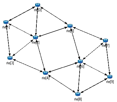
Figure: The network

The corresponding NED description would look like this:

// // A network // network Network {     submodules:         node1: Node;         node2: Node;         node3: Node;         ...     connections:         node1.port++ <--> {datarate=100Mbps;} <--> node2.port++;         node2.port++ <--> {datarate=100Mbps;} <--> node4.port++;         node4.port++ <--> {datarate=100Mbps;} <--> node6.port++;         ... }

The above code defines a network type named Network. Note that the NED language uses the familiar curly brace syntax, and "//" to denote comments.

NOTE

JavaDoc

Doxygen

The network contains several nodes, named node1, node2, etc. from the NED module type Node. We'll define Node in the next sections.

The second half of the declaration defines how the nodes are to be connected. The double arrow means bidirectional connection. The connection points of modules are called gates, and the port++ notation adds a new gate to the port[] gate vector. Gates and connections will be covered in more detail in sections [3.7] and [3.9]. Nodes are connected with a channel that has a data rate of 100Mbps.

NOTE

ports

gate

port

The above code would be placed into a file named Net6.ned. It is a convention to put every NED definition into its own file and to name the file accordingly, but it is not mandatory to do so.

One can define any number of networks in the NED files, and for every simulation the user has to specify which network to set up. The usual way of specifying the network is to put the network option into the configuration (by default the omnetpp.ini file):

[General] network = Network

3.2.2 Introducing a Channel¶

It is cumbersome to have to repeat the data rate for every connection. Luckily, NED provides a convenient solution: one can create a new channel type that encapsulates the data rate setting, and this channel type can be defined inside the network so that it does not litter the global namespace.

The improved network will look like this:

// // A Network // network Network {     types:         channel C extends ned.DatarateChannel {             datarate = 100Mbps;         }     submodules:         node1: Node;         node2: Node;         node3: Node;         ...     connections:         node1.port++ <--> C <--> node2.port++;         node2.port++ <--> C <--> node4.port++;         node4.port++ <--> C <--> node6.port++;         ... }

Later sections will cover the concepts used (inner types, channels, the DatarateChannel built-in type, inheritance) in detail.

3.2.3 The App, Routing, and Queue Simple Modules¶

Simple modules are the basic building blocks for other (compound) modules, denoted by the simple keyword. All active behavior in the model is encapsulated in simple modules. Behavior is defined with a C++ class; NED files only declare the externally visible interface of the module (gates, parameters).

In our example, we could define Node as a simple module. However, its functionality is quite complex (traffic generation, routing, etc), so it is better to implement it with several smaller simple module types which we are going to assemble into a compound module. We'll have one simple module for traffic generation (App), one for routing (Routing), and one for queueing up packets to be sent out (Queue). For brevity, we omit the bodies of the latter two in the code below.

simple App {     parameters:         int destAddress;         ...         @display("i=block/browser");     gates:         input in;         output out; }  simple Routing {     ... }  simple Queue {     ... }

By convention, the above simple module declarations go into the App.ned, Routing.ned and Queue.ned files.

NOTE

App

Routing

Queue

Let us look at the first simple module type declaration. App has a parameter called destAddress (others have been omitted for now), and two gates named out and in for sending and receiving application packets.

The argument of @display() is called a display string, and it defines the rendering of the module in graphical environments; "i=..." defines the default icon.

Generally, @-words like @display are called properties in NED, and they are used to annotate various objects with metadata. Properties can be attached to files, modules, parameters, gates, connections, and other objects, and parameter values have a very flexible syntax.

3.2.4 The Node Compound Module¶

Now we can assemble App, Routing and Queue into the compound module Node. A compound module can be thought of as a "cardboard box" that groups other modules into a larger unit, which can further be used as a building block for other modules; networks are also a kind of compound module.

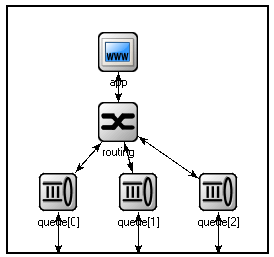
Figure: The Node compound module

module Node {     parameters:         int address;         @display("i=misc/node_vs,gold");     gates:         inout port[];     submodules:         app: App;         routing: Routing;         queue[sizeof(port)]: Queue;     connections:         routing.localOut --> app.in;         routing.localIn <-- app.out;         for i=0..sizeof(port)-1 {             routing.out[i] --> queue[i].in;             routing.in[i] <-- queue[i].out;             queue[i].line <--> port[i];         } }

Compound modules, like simple modules, may have parameters and gates. Our Node module contains an address parameter, plus a gate vector of unspecified size, named port. The actual gate vector size will be determined implicitly by the number of neighbours when we create a network from nodes of this type. The type of port[] is inout, which allows bidirectional connections.

The modules that make up the compound module are listed under submodules . Our Node compound module type has an app and a routing submodule, plus a queue[] submodule vector that contains one Queue module for each port, as specified by [sizeof(port)]. (It is legal to refer to [sizeof(port)] because the network is built in top-down order, and the node is already created and connected at network level when its submodule structure is built out.)

In the connections section, the submodules are connected to each other and to the parent module. Single arrows are used to connect input and output gates, and double arrows connect inout gates, and a for loop is utilized to connect the routing module to each queue module, and to connect the outgoing/incoming link (line gate) of each queue to the corresponding port of the enclosing module.

3.2.5 Putting It Together¶

We have created the NED definitions for this example, but how are they used by OMNeT++? When the simulation program is started, it loads the NED files. The program should already contain the C++ classes that implement the needed simple modules, App, Routing and Queue; their C++ code is either part of the executable or is loaded from a shared library. The simulation program also loads the configuration (omnetpp.ini), and determines from it that the simulation model to be run is the Network network. Then the network is instantiated for simulation.

The simulation model is built in a top-down preorder fashion. This means that starting from an empty system module, all submodules are created, their parameters and gate vector sizes are assigned, and they are fully connected before the submodule internals are built.

* * *

In the following sections we'll go through the elements of the NED language and look at them in more detail.

3.3 Simple Modules¶

Simple modules are the active components in the model. Simple modules are defined with the simple keyword.

An example simple module:

simple Queue {     parameters:         int capacity;         @display("i=block/queue");     gates:         input in;         output out; }

Both the parameters and gates sections are optional, that is, they can be left out if there is no parameter or gate. In addition, the parameters keyword itself is optional too; it can be left out even if there are parameters or properties.

Note that the NED definition doesn't contain any code to define the operation of the module: that part is expressed in C++. By default, OMNeT++ looks for C++ classes of the same name as the NED type (so here, Queue).

One can explicitly specify the C++ class with the @class property. Classes with namespace qualifiers are also accepted, as shown in the following example that uses the mylib::Queue class:

simple Queue {     parameters:         int capacity;         @class(mylib::Queue);         @display("i=block/queue");     gates:         input in;         output out; }

If there are several modules whose C++ implementation classes are in the same namespace, a better alternative to @class is the @namespace property. The C++ namespace given with @namespace will be prepended to the normal class name. In the following example, the C++ classes will be mylib::App, mylib::Router and mylib::Queue:

@namespace(mylib);  simple App {    ... }  simple Router {    ... }  simple Queue {    ... }

The @namespace property may not only be specified at file level as in the above example, but for packages as well. When placed in a file called package.ned, the namespace will apply to all components in that package and below.

The implementation C++ classes need to be subclassed from the cSimpleModule library class; chapter [4] of this manual describes in detail how to write them.

Simple modules can be extended (or specialized) via subclassing. The motivation for subclassing can be to set some open parameters or gate sizes to a fixed value (see [3.6] and [3.7]), or to replace the C++ class with a different one. Now, by default, the derived NED module type will inherit the C++ class from its base, so it is important to remember that you need to write out @class if you want it to use the new class.

The following example shows how to specialize a module by setting a parameter to a fixed value (and leaving the C++ class unchanged):

simple Queue {    int capacity;    ... }  simple BoundedQueue extends Queue {    capacity = 10; }

In the next example, the author wrote a PriorityQueue C++ class, and wants to have a corresponding NED type, derived from Queue. However, it does not work as expected:

simple PriorityQueue extends Queue // wrong! still uses the Queue C++ class { }

The correct solution is to add a @class property to override the inherited C++ class:

simple PriorityQueue extends Queue {    @class(PriorityQueue); }

Inheritance in general will be discussed in section [3.13].

3.4 Compound Modules¶

A compound module groups other modules into a larger unit. A compound module may have gates and parameters like a simple module, but no active behavior is associated with it.

[Although the C++ class for a compound module can be overridden with the @class property, this is a feature that should probably never be used. Encapsulate the code into a simple module, and add it as a submodule.]

NOTE

A compound module declaration may contain several sections, all of them optional:

module Host {    types:        ...    parameters:        ...    gates:        ...    submodules:        ...    connections:        ... }

Modules contained in a compound module are called submodules, and they are listed in the submodules section. One can create arrays of submodules (i.e. submodule vectors), and the submodule type may come from a parameter.

Connections are listed under the connections section of the declaration. One can create connections using simple programming constructs (loop, conditional). Connection behaviour can be defined by associating a channel with the connection; the channel type may also come from a parameter.

Module and channel types only used locally can be defined in the types section as inner types, so that they do not pollute the namespace.

Compound modules may be extended via subclassing. Inheritance may add new submodules and new connections as well, not only parameters and gates. Also, one may refer to inherited submodules, to inherited types etc. What is not possible is to "de-inherit" or modify submodules or connections.

[With one exception: Since OMNeT++ version 5.6, reconnecting existing gates is possible using the reconnect property, see [3.9.2].]

In the following example, we show how to assemble common protocols into a "stub" for wireless hosts, and add user agents via subclassing.

[Module types, gate names, etc. used in this chapter's code examples are entirely made-up, and not based on an actual OMNeT++-based model framework]

module WirelessHostBase {    gates:        input radioIn;    submodules:        tcp: TCP;        ip: IP;        wlan: Ieee80211;    connections:        tcp.ipOut --> ip.tcpIn;        tcp.ipIn <-- ip.tcpOut;        ip.nicOut++ --> wlan.ipIn;        ip.nicIn++ <-- wlan.ipOut;        wlan.radioIn <-- radioIn; }  module WirelessHost extends WirelessHostBase {    submodules:        webAgent: WebAgent;    connections:        webAgent.tcpOut --> tcp.appIn++;        webAgent.tcpIn <-- tcp.appOut++; }

The WirelessHost compound module can further be extended, for example with an Ethernet port:

module DesktopHost extends WirelessHost {    gates:        inout ethg;    submodules:        eth: EthernetNic;    connections:        ip.nicOut++ --> eth.ipIn;        ip.nicIn++ <-- eth.ipOut;        eth.phy <--> ethg; }

3.5 Channels¶

Channels encapsulate parameters and behaviour associated with connections. Channels are like simple modules, in the sense that there are C++ classes behind them. The rules for finding the C++ class for a NED channel type is the same as with simple modules: the default class name is the NED type name unless there is a @class property ( @namespace is also recognized), and the C++ class is inherited when the channel is subclassed.

Thus, the following channel type would expect a CustomChannel C++ class to be present:

channel CustomChannel  // requires a CustomChannel C++ class { }

The practical difference compared to modules is that one rarely needs to write custom channel C++ class because there are predefined channel types that one can subclass from, inheriting their C++ code. The predefined types are: ned.IdealChannel, ned.DelayChannel and ned.DatarateChannel. ("ned" is the package name; one can get rid of it by importing the types with the import ned.* directive. Packages and imports are described in section [3.14].)

IdealChannel has no parameters, and lets through all messages without delay or any side effect. A connection without a channel object and a connection with an IdealChannel behave in the same way. Still, IdealChannel has its uses, for example when a channel object is required so that it can carry a new property or parameter that is going to be read by other parts of the simulation model.

DelayChannel has two parameters:

delay is a double parameter which represents the propagation delay of the message. Values need to be specified together with a time unit (s, ms, us, etc.)
disabled is a boolean parameter that defaults to false; when set to true, the channel object will drop all messages.

DatarateChannel has a few additional parameters compared to DelayChannel:

datarate is a double parameter that represents the data rate of the channel. Values need to be specified in bits per second or its multiples as unit (bps, kbps, Mbps, Gbps, etc.) Zero is treated specially and results in zero transmission duration, i.e. it stands for infinite bandwidth. Zero is also the default. Data rate is used for calculating the transmission duration of packets.
ber and per stand for Bit Error Rate and Packet Error Rate, and allow basic error modelling. They expect a double in the [0,1] range. When the channel decides (based on random numbers) that an error occurred during transmission of a packet, it sets an error flag in the packet object. The receiver module is expected to check the flag, and discard the packet as corrupted if it is set. The default ber and per are zero.

NOTE

setDeliverOnReceptionStart()

cGate

The following example shows how to create a new channel type by specializing DatarateChannel:

channel Ethernet100 extends ned.DatarateChannel {     datarate = 100Mbps;     delay = 100us;     ber = 1e-10; }

NOTE

One may add parameters and properties to channels via subclassing, and may modify existing ones. In the following example, we introduce distance-based calculation of the propagation delay:

channel DatarateChannel2 extends ned.DatarateChannel {     double distance @unit(m);     delay = this.distance / 200000km * 1s; }

Parameters are primarily intended to be read by the underlying C++ class, but new parameters may also be added as annotations to be used by other parts of the model. For example, a cost parameter may be used for routing decisions in routing module, as shown in the example below. The example also shows annotation using properties ( @backbone ).

channel Backbone extends ned.DatarateChannel {     @backbone;     double cost = default(1); }

3.6 Parameters¶

Parameters are variables that belong to a module. Parameters can be used in building the topology (number of nodes, etc), and to supply input to C++ code that implements simple modules and channels.

Parameters can be of type double , int , bool , string and xml ; they can also be declared volatile . For the numeric types, a unit of measurement can also be specified ( @unit property), to increase type safety.

Parameters can get their value from NED files or from the configuration (omnetpp.ini). A default value can also be given (default(...)), which is used if the parameter is not assigned otherwise.

The following example shows a simple module that has five parameters, three of which have default values:

simple App {     parameters:         string protocol;       // protocol to use: "UDP" / "IP" / "ICMP" / ...         int destAddress;       // destination address         volatile double sendInterval @unit(s) = default(exponential(1s));                                // time between generating packets         volatile int packetLength @unit(byte) = default(100B);                                // length of one packet         volatile int timeToLive = default(32);                                // maximum number of network hops to survive     gates:         input in;         output out; }

3.6.1 Assigning a Value¶

Parameters may get their values in several ways: from NED code, from the configuration (omnetpp.ini), or even, interactively from the user. NED lets one assign parameters at several places: in subclasses via inheritance; in submodule and connection definitions where the NED type is instantiated; and in networks and compound modules that directly or indirectly contain the corresponding submodule or connection.

For instance, one could specialize the above App module type via inheritance with the following definition:

simple PingApp extends App {     parameters:         protocol = "ICMP/ECHO"         sendInterval = default(1s);         packetLength = default(64byte); }

This definition sets the protocol parameter to a fixed value ("ICMP/ECHO"), and changes the default values of the sendInterval and packetLength parameters. protocol is now locked down in PingApp, its value cannot be modified via further subclassing or other ways. sendInterval and packetLength are still unassigned here, only their default values have been overwritten.

Now, let us see the definition of a Host compound module that uses PingApp as submodule:

module Host {     submodules:         ping : PingApp {             packetLength = 128B; // always ping with 128-byte packets         }         ... }

This definition sets the packetLength parameter to a fixed value. It is now hardcoded that Hosts send 128-byte ping packets; this setting cannot be changed from NED or the configuration.

It is not only possible to set a parameter from the compound module that contains the submodule, but also from modules higher up in the module tree. A network that employs several Host modules could be defined like this:

network Network {     submodules:         host[100]: Host {             ping.timeToLive = default(3);             ping.destAddress = default(0);         }         ... }

Parameter assignment can also be placed into the parameters block of the parent compound module, which provides additional flexibility. The following definition sets up the hosts so that half of them pings host #50, and the other half pings host #0:

network Network {     parameters:         host[*].ping.timeToLive = default(3);         host[0..49].ping.destAddress = default(50);         host[50..].ping.destAddress = default(0);      submodules:         host[100]: Host;         ... }

Note the use of asterisk to match any index, and .. to match index ranges.

If there were a number of individual hosts instead of a submodule vector, the network definition could look like this:

network Network {     parameters:         host*.ping.timeToLive = default(3);         host{0..49}.ping.destAddress = default(50);         host{50..}.ping.destAddress = default(0);      submodules:         host0: Host;         host1: Host;         host2: Host;         ...         host99: Host; }

An asterisk matches any substring not containing a dot, and a .. within a pair of curly braces matches a natural number embedded in a string.

In most assigments we have seen above, the left hand side of the equal sign contained a dot and often a wildcard as well (asterisk or numeric range); we call these assignments pattern assignments or deep assignments.

There is one more wildcard that can be used in pattern assignments, and this is the double asterisk; it matches any sequence of characters including dots, so it can match multiple path elements. An example:

network Network {     parameters:         **.timeToLive = default(3);         **.destAddress = default(0);     submodules:         host0: Host;         host1: Host;         ... }

Note that some assignments in the above examples changed default values, while others set parameters to fixed values. Parameters that received no fixed value in the NED files can be assigned from the configuration (omnetpp.ini).

IMPORTANT

A parameter can be assigned in the configuration using a similar syntax as NED pattern assignments (actually, it would be more historically accurate to say it the other way round, that NED pattern assignments use a similar syntax to ini files):

Network.host[*].ping.sendInterval = 500ms  # for the host[100] example Network.host*.ping.sendInterval = 500ms    # for the host0,host1,... example **.sendInterval = 500ms

One often uses the double asterisk to save typing. One can write

**.ping.sendInterval = 500ms

Or if one is certain that only ping modules have sendInterval parameters, the following will suffice:

**.sendInterval = 500ms

Parameter assignments in the configuration are described in section [10.3].

One can also write expressions, including stochastic expressions, in NED files and in ini files as well. For example, here's how one can add jitter to the sending of ping packets:

**.sendInterval = 1s + normal(0s, 0.001s)  # or just: normal(1s, 0.001s)

If there is no assignment for a parameter in NED or in the ini file, the default value (given with =default(...) in NED) will be applied implicitly. If there is no default value, the user will be asked, provided the simulation program is allowed to do that; otherwise there will be an error. (Interactive mode is typically disabled for batch executions where it would do more harm than good.)

It is also possible to explicitly apply the default (this can sometimes be useful):

**.sendInterval = default

Finally, one can explicitly ask the simulator to prompt the user interactively for the value (again, provided that interactivity is enabled; otherwise this will result in an error):

**.sendInterval = ask

NOTE

model

experiments

3.6.2 Expressions¶

Parameter values may be given with expressions. NED language expressions have a C-like syntax, with some variations on operator names: binary and logical XOR are # and ##, while ^ has been reassigned to power-of instead. The + operator does string concatenation as well as numeric addition. Expressions can use various numeric, string, stochastic and other functions (fabs(), toUpper(), uniform(), erlang_k(), etc.).

NOTE

Expressions may refer to module parameters, gate vector and module vector sizes (using the sizeof operator) and the index of the current module in a submodule vector ( index ).

Expressions may refer to parameters of the compound module being defined, of the current module (with the this. prefix), and to parameters of already defined submodules, with the syntax submodule.parametername (or submodule[index].parametername).

3.6.3 volatile¶

The volatile modifier causes the parameter's value expression to be evaluated every time the parameter is read. This has significance if the expression is not constant, for example it involves numbers drawn from a random number generator. In contrast, non-volatile parameters are evaluated only once. (This practically means that they are evaluated and replaced with the resulting constant at the start of the simulation.)

To better understand volatile , let's suppose we have a Queue simple module that has a volatile double parameter named serviceTime.

simple Queue {     parameters:         volatile double serviceTime; }

Because of the volatile modifier, the queue module's C++ implementation is expected to re-read the serviceTime parameter whenever a value is needed; that is, for every job serviced. Thus, if serviceTime is assigned an expression like uniform(0.5s, 1.5s), every job will have a different, random service time. To highlight this effect, here's how one can have a time-varying parameter by exploiting the simTime() NED function that returns the current simulation time:

**.serviceTime = simTime()<1000s ? 1s : 2s  # queue that slows down after 1000s

In practice, a volatile parameters are typically used as a configurable source of random numbers for modules.

NOTE

uniform(0.5s, 1.5s)

1.2975367s

3.6.4 Units¶

One can declare a parameter to have an associated unit of measurement, by adding the @unit property. An example:

simple App {     parameters:         volatile double sendInterval @unit(s) = default(exponential(350ms));         volatile int packetLength @unit(byte) = default(4KiB);     ... }

The @unit(s) and @unit(byte) declarations specify the measurement unit for the parameter. Values assigned to parameters must have the same or compatible unit, i.e. @unit(s) accepts milliseconds, nanoseconds, minutes, hours, etc., and @unit(byte) accepts kilobytes, megabytes, etc. as well.

NOTE

bogomips

The OMNeT++ runtime does a full and rigorous unit check on parameters to ensure "unit safety" of models. Constants should always include the measurement unit.

The @unit property of a parameter cannot be added or overridden in subclasses or in submodule declarations.

3.6.5 XML Parameters¶

Sometimes modules need complex data structures as input, which is something that cannot be done well with module parameters. One solution is to place the input data into a custom configuration file, pass the file name to the module in a string parameter, and let the module read and parse the file.

It is somewhat easier if the configuration uses XML syntax, because OMNeT++ contains built-in support for XML files. Using an XML parser (LibXML2 or Expat), OMNeT++ reads and DTD-validates the file (if the XML document contains a DOCTYPE), caches the file (so that references to it from several modules will result in the file being loaded only once), allows selection of parts of the document using an XPath-subset notation, and presents the contents in a DOM-like object tree.

This capability can be accessed via the NED parameter type xml , and the xmldoc() function. One can point xml -type module parameters to a specific XML file (or to an element inside an XML file) via the xmldoc() function. One can assign xml parameters both from NED and from omnetpp.ini.

The following example declares an xml parameter, and assigns an XML file to it. The file name is understood as being relative to the working directory.

simple TrafGen {     parameters:         xml profile;     gates:         output out; }  module Node {     submodules:         trafGen1 : TrafGen {             profile = xmldoc("data.xml");         }         ... }

xmldoc() also lets one select an element within an XML file. In case one has a model that contains numerous modules that need XML input, this feature allows the user get rid of the countless small XML files by aggregating them into a single XML file. For example, the following XML file contains two profiles identified with the IDs gen1 and gen2:

<?xml> <root>     <profile id="gen1">           <param>3</param>           <param>5</param>     </profile>     <profile id="gen2">           <param>9</param>     </profile> </root>

And one can assign each profile to a corresponding submodule using an XPath-like expression:

module Node {     submodules:         trafGen1 : TrafGen {             profile = xmldoc("all.xml", "/root/profile[@id='gen1']");         }         trafGen2 : TrafGen {             profile = xmldoc("all.xml", "/root/profile[@id='gen2']");         } }

It is also possible to create an XML document from a string constant, using the xml() function. This is especially useful for creating a default value for xml parameters. An example:

simple TrafGen {     parameters:         xml profile = xml("<root/>"); // empty document as default         ... }

The xml() function, like xmldoc() , also supports an optional second XPath parameter for selecting a subtree.

3.7 Gates¶

Gates are the connection points of modules. OMNeT++ has three types of gates: input, output and inout, the latter being essentially an input and an output gate glued together.

A gate, whether input or output, can only be connected to one other gate. (For compound module gates, this means one connection "outside" and one "inside".) It is possible, though generally not recommended, to connect the input and output sides of an inout gate separately (see section [3.9]).

One can create single gates and gate vectors. The size of a gate vector can be given inside square brackets in the declaration, but it is also possible to leave it open by just writing a pair of empty brackets ("[]").

When the gate vector size is left open, one can still specify it later, when subclassing the module, or when using the module for a submodule in a compound module. However, it does not need to be specified because one can create connections with the gate++ operator that automatically expands the gate vector.

The gate size can be queried from various NED expressions with the sizeof() operator.

NED normally requires that all gates be connected. To relax this requirement, one can annotate selected gates with the @loose property, which turns off the connectivity check for that gate. Also, input gates that solely exist so that the module can receive messages via sendDirect() (see [4.7.5]) should be annotated with @directIn . It is also possible to turn off the connectivity check for all gates within a compound module by specifying the allowunconnected keyword in the module's connections section.

Let us see some examples.

In the following example, the Classifier module has one input for receiving jobs, which it will send to one of the outputs. The number of outputs is determined by a module parameter:

simple Classifier {     parameters:         int numCategories;     gates:         input in;         output out[numCategories]; }

The following Sink module also has its in[] gate defined as a vector, so that it can be connected to several modules:

simple Sink {     gates:         input in[]; }

The following lines define a node for building a square grid. Gates around the edges of the grid are expected to remain unconnected, hence the @loose annotation:

simple GridNode {     gates:         inout neighbour[4] @loose; }

WirelessNode below is expected to receive messages (radio transmissions) via direct sending, so its radioIn gate is marked with @directIn .

simple WirelessNode {     gates:         input radioIn @directIn; }

In the following example, we define TreeNode as having gates to connect any number of children, then subclass it to get a BinaryTreeNode to set the gate size to two:

simple TreeNode {     gates:         inout parent;         inout children[]; }  simple BinaryTreeNode extends TreeNode {     gates:         children[2]; }

An example for setting the gate vector size in a submodule, using the same TreeNode module type as above:

module BinaryTree {     submodules:         nodes[31]: TreeNode {             gates:                 children[2];         }     connections:         ... }

3.8 Submodules¶

Modules that a compound module is composed of are called its submodules. A submodule has a name, and it is an instance of a compound or simple module type. In the NED definition of a submodule, this module type is usually given statically, but it is also possible to specify the type with a string expression. (The latter feature, parametric submodule types, will be discussed in section [3.11.1].)

NED supports submodule arrays (vectors) and conditional submodules as well. Submodule vector size, unlike gate vector size, must always be specified and cannot be left open as with gates.

It is possible to add new submodules to an existing compound module via subclassing; this has been described in the section [3.4].

The basic syntax of submodules is shown below:

module Node {     submodules:         routing: Routing;   // a submodule         queue[sizeof(port)]: Queue;  // submodule vector         ... }

As already seen in previous code examples, a submodule may also have a curly brace block as body, where one can assign parameters, set the size of gate vectors, and add/modify properties like the display string ( @display ). It is not possible to add new parameters and gates.

Display strings specified here will be merged with the display string from the type to get the effective display string. The merge algorithm is described in chapter [8].

module Node {     gates:         inout port[];     submodules:         routing: Routing {             parameters:   // this keyword is optional                 routingTable = "routingtable.txt"; // assign parameter             gates:                 in[sizeof(port)];  // set gate vector size                 out[sizeof(port)];         }         queue[sizeof(port)]: Queue {             @display("t=queue id $id"); // modify display string             id = 1000+index;  // use submodule index to generate different IDs         }     connections:         ... }

An empty body may be omitted, that is,

          queue: Queue;

is the same as

          queue: Queue {       }

A submodule or submodule vector can be conditional. The if keyword and the condition itself goes after the submodule type, like in the example below:

module Host {     parameters:         bool withTCP = default(true);     submodules:         tcp : TCP if withTCP;         ... }

Note that with submodule vectors, setting zero vector size can be used as an alternative to the if condition.

3.9 Connections¶

Connections are defined in the connections section of compound modules. Connections cannot span across hierarchy levels; one can connect two submodule gates, a submodule gate and the "inside" of the parent (compound) module's gates, or two gates of the parent module (though this is rarely useful), but it is not possible to connect to any gate outside the parent module, or inside compound submodules.

Input and output gates are connected with a normal arrow, and inout gates with a double-headed arrow "<-->". To connect the two gates with a channel, use two arrows and put the channel specification in between. The same syntax is used to add properties such as @display to the connection.

Some examples have already been shown in the NED Quickstart section ([3.2]); let's see some more.

It has been mentioned that an inout gate is basically an input and an output gate glued together. These sub-gates can also be addressed (and connected) individually if needed, as port$i and port$o (or for vector gates, as port$i[$k$] and port$o[k]).

Gates are specified as modulespec.gatespec (to connect a submodule), or as gatespec (to connect the compound module). modulespec is either a submodule name (for scalar submodules), or a submodule name plus an index in square brackets (for submodule vectors). For scalar gates, gatespec is the gate name; for gate vectors it is either the gate name plus an index in square brackets, or gatename ++.

The gatename ++ notation causes the first unconnected gate index to be used. If all gates of the given gate vector are connected, the behavior is different for submodules and for the enclosing compound module. For submodules, the gate vector expands by one. For a compound module, after the last gate is connected, ++ will stop with an error.

NOTE

When the ++ operator is used with $i or $o (e.g. g$i++ or g$o++, see later), it will actually add a gate pair (input+output) to maintain equal gate sizes for the two directions.

3.9.1 Channel Specification¶

Channel specifications (-->channelspec--> inside a connection) are similar to submodules in many respect. Let's see some examples!

The following connections use two user-defined channel types, Ethernet100 and Backbone. The code shows the syntax for assigning parameters (cost and length) and specifying a display string (and NED properties in general):

a.g++ <--> Ethernet100 <--> b.g++; a.g++ <--> Backbone {cost=100; length=52km; ber=1e-8;} <--> b.g++; a.g++ <--> Backbone {@display("ls=green,2");} <--> b.g++;

When using built-in channel types, the type name can be omitted; it will be inferred from the parameter names.

a.g++ <--> {delay=10ms;} <--> b.g++; a.g++ <--> {delay=10ms; ber=1e-8;} <--> b.g++; a.g++ <--> {@display("ls=red");} <--> b.g++;

If datarate, ber or per is assigned, ned.DatarateChannel will be chosen. Otherwise, if delay or disabled is present, it will be ned.DelayChannel; otherwise it is ned.IdealChannel. Naturally, if other parameter names are assigned in a connection without an explicit channel type, it will be an error (with "ned.DelayChannel has no such parameter" or similar message).

Connection parameters, similarly to submodule parameters, can also be assigned using pattern assignments, albeit the channel names to be matched with patterns are a little more complicated and less convenient to use. A channel can be identified with the name of its source gate plus the channel name; the channel name is currently always channel. It is illustrated by the following example:

module Queueing {     parameters:         source.out.channel.delay = 10ms;         queue.out.channel.delay = 20ms;     submodules:         source: Source;         queue: Queue;         sink: Sink;     connections:         source.out --> ned.DelayChannel --> queue.in;         queue.out --> ned.DelayChannel <--> sink.in;

Using bidirectional connections is a bit trickier, because both directions must be covered separately:

network Network {     parameters:         hostA.g$o[0].channel.datarate = 100Mbps; // the A -> B connection         hostB.g$o[0].channel.datarate = 100Mbps; // the B -> A connection         hostA.g$o[1].channel.datarate = 1Gbps;   // the A -> C connection         hostC.g$o[0].channel.datarate = 1Gbps;   // the C -> A connection     submodules:         hostA: Host;         hostB: Host;         hostC: Host;     connections:         hostA.g++ <--> ned.DatarateChannel <--> hostB.g++;         hostA.g++ <--> ned.DatarateChannel <--> hostC.g++;

Also, with the ++ syntax it is not always easy to figure out which gate indices map to the connections one needs to configure. If connection objects could be given names to override the default name "channel", that would make it easier to identify connections in patterns. This feature is described in the next section.

3.9.2 Reconnecting Gates¶

Normally, it is an error for NED connection to refer to a gate which is already connected. This behavior can be overridden with the @reconnect property. A syntax example:

a.out --> {@reconnect;} --> b.in;

When a connection with the @reconnect property is encountered by the network builder, it first checks whether any of the involved gates are connected. If they are, it will unconnect them before proceeding to create the new connection.

The usefulness of @reconnect lies with inheritance, as it allows one to modify connections in the base compound module. For example, it is possible to insert a new submodule in the path between two connected submodules, which eliminates the need for "hook" submodules in compound modules that are meant to be very configurable. This is illustrated in the following example:

module Base {     submodules:         a: A;         b: B;     connections:         a.out --> b.in; }  module Derived extends Base {     submodules:         c: C; // inserted between a and b     connections:         a.out --> {@reconnect;} --> c.in;         c.out --> {@reconnect;} --> b.in; }

3.9.3 Channel Names¶

The default name given to channel objects is "channel". Since OMNeT++ 4.3 it is possible to specify the name explicitly, and also to override the default name per channel type. The purpose of custom channel names is to make addressing easier when channel parameters are assigned from ini files.

The syntax for naming a channel in a connection is similar to submodule syntax: name: type. Since both name and type are optional, the colon must be there after name even if type is missing, in order to remove the ambiguity.

Examples:

r1.pppg++ <--> eth1: EthernetChannel <--> r2.pppg++; a.out --> foo: {delay=1ms;} --> b.in; a.out --> bar: --> b.in;

In the absence of an explicit name, the channel name comes from the @defaultname property of the channel type if that exists.

channel Eth10G extends ned.DatarateChannel like IEth {     @defaultname(eth10G); }

There's a catch with @defaultname though: if the channel type is specified with a **.channelname.liketype= line in an ini file, then the channel type's @defaultname cannot be used as channelname in that configuration line, because the channel type would only be known as a result of using that very configuration line. To illustrate the problem, consider the above Eth10G channel, and a compound module containing the following connection:

r1.pppg++ <--> <> like IEth <--> r2.pppg++;

Then consider the following inifile:

**.eth10G.typename = "Eth10G"   # Won't match! The eth10G name would come from                                 #   the Eth10G type - catch-22! **.channel.typename = "Eth10G"  # OK, as lookup assumes the name "channel" **.eth10G.datarate = 10.01Gbps  # OK, channel already exists with name "eth10G"

The anomaly can be avoided by using an explicit channel name in the connection, not using @defaultname, or by specifying the type via a module parameter (e.g. writing <param> like ... instead of <> like ...).

3.10 Multiple Connections¶

Simple programming constructs (loop, conditional) allow creating multiple connections easily.

This will be shown in the following examples.

3.10.1 Examples¶

3.10.1.1 Chain¶

One can create a chain of modules like this:

module Chain     parameters:         int count;     submodules:         node[count] : Node {             gates:                 port[2];         }     connections allowunconnected:         for i = 0..count-2 {             node[i].port[1] <--> node[i+1].port[0];         } }

3.10.1.2 Binary Tree¶

One can build a binary tree in the following way:

simple BinaryTreeNode {     gates:         inout left;         inout right;         inout parent; }  module BinaryTree {     parameters:         int height;     submodules:         node[2^height-1]: BinaryTreeNode;     connections allowunconnected:         for i=0..2^(height-1)-2 {             node[i].left <--> node[2*i+1].parent;             node[i].right <--> node[2*i+2].parent;         } }

Note that not every gate of the modules will be connected. By default, an unconnected gate produces a run-time error message when the simulation is started, but this error message is turned off here with the allowunconnected modifier. Consequently, it is the simple modules' responsibility not to send on an unconnected gate.

3.10.1.3 Random Graph¶

Conditional connections can be used to generate random topologies , for example. The following code generates a random subgraph of a full graph:

module RandomGraph {     parameters:         int count;         double connectedness; // 0.0<x<1.0     submodules:         node[count]: Node {             gates:                 in[count];                 out[count];         }     connections allowunconnected:         for i=0..count-1, for j=0..count-1 {             node[i].out[j] --> node[j].in[i]                 if i!=j && uniform(0,1)<connectedness;         } }

Note the use of the allowunconnected modifier here too, to turn off error messages produced by the network setup code for unconnected gates.

3.10.2 Connection Patterns¶

Several approaches can be used for creating complex topologies that have a regular structure; three of them are described below.

3.10.2.1 "Subgraph of a Full Graph"¶

This pattern takes a subset of the connections of a full graph. A condition is used to "carve out" the necessary interconnection from the full graph:

for i=0..N-1, for j=0..N-1 {     node[i].out[...] --> node[j].in[...] if condition(i,j); }

The RandomGraph compound module (presented earlier) is an example of this pattern, but the pattern can generate any graph where an appropriate condition(i,j) can be formulated. For example, when generating a tree structure, the condition would return whether node j is a child of node i or vice versa.

Though this pattern is very general, its usage can be prohibitive if the number of nodes N is high and the graph is sparse (it has much less than N² connections). The following two patterns do not suffer from this drawback.

3.10.2.2 "Connections of Each Node"¶

The pattern loops through all nodes and creates the necessary connections for each one. It can be generalized like this:

for i=0..Nnodes, for j=0..Nconns(i)-1 {     node[i].out[j] --> node[rightNodeIndex(i,j)].in[j]; }

The Hypercube compound module (to be presented later) is a clear example of this approach. BinaryTree can also be regarded as an example of this pattern where the inner j loop is unrolled.

The applicability of this pattern depends on how easily the rightNodeIndex(i,j) function can be formulated.

3.10.2.3 "Enumerate All Connections"¶

A third pattern is to list all connections within a loop:

for i=0..Nconnections-1 {     node[leftNodeIndex(i)].out[...] --> node[rightNodeIndex(i)].in[...]; }

This pattern can be used if leftNodeIndex(i) and rightNodeIndex(i) mapping functions can be sufficiently formulated.

The Chain module is an example of this approach where the mapping functions are extremely simple: leftNodeIndex(i)=i and rightNodeIndex(i) = i+1. The pattern can also be used to create a random subset of a full graph with a fixed number of connections.

In the case of irregular structures where none of the above patterns can be employed, one can resort to listing all connections, like one would do it in most existing simulators.

3.11 Parametric Submodule and Connection Types¶

3.11.1 Parametric Submodule Types¶

A submodule type may be specified with a module parameter of the type string , or in general, with any string-typed expression. The syntax uses the like keyword.

Let us begin with an example:

network Net6 {     parameters:         string nodeType;     submodules:         node[6]: <nodeType> like INode {             address = index;         }     connections:         ... }

It creates a submodule vector whose module type will come from the nodeType parameter. For example, if nodeType is set to "SensorNode", then the module vector will consist of sensor nodes, provided such module type exists and it qualifies. What this means is that the INode must be an existing module interface, which the SensorNode module type must implement (more about this later).

As already mentioned, one can write an expression between the angle brackets. The expression may use the parameters of the parent module and of previously defined submodules, and has to yield a string value. For example, the following code is also valid:

network Net6 {     parameters:         string nodeTypePrefix;         int variant;     submodules:         node[6]: <nodeTypePrefix + "Node" + string(variant)> like INode {            ... }

The corresponding NED declarations:

moduleinterface INode {     parameters:         int address;     gates:         inout port[]; }  module SensorNode like INode {     parameters:         int address;         ...     gates:         inout port[];         ... }

The "<nodeType> like INode" syntax has an issue when used with submodule vectors: does not allow one to specify different types for different indices. The following syntax is better suited for submodule vectors:

The expression between the angle brackets may be left out altogether, leaving a pair of empty angle brackets, <>:

module Node {     submodules:         nic: <> like INic;  // type name expression left unspecified         ... }

Now the submodule type name is expected to be defined via typename pattern assignments. Typename pattern assignments look like pattern assignments for the submodule's parameters, only the parameter name is replaced by the typename keyword. Typename pattern assignments may also be written in the configuration file. In a network that uses the above Node NED type, typename pattern assignments would look like this:

network Network {     parameters:         node[*].nic.typename = "Ieee80211g";     submodules:         node: Node[100]; }

A default value may also be specified between the angle brackets; it will be used if there is no typename assignment for the module:

module Node {     submodules:         nic: <default("Ieee80211b")> like INic;         ... }

There must be exactly one module type that goes by the simple name Ieee80211b and also implements the module interface INic, otherwise an error message will be issued. (The imports in Node's the NED file play no role in the type resolution.) If there are two or more such types, one can remove the ambiguity by specifying the fully qualified module type name, i.e. one that also includes the package name:

module Node {     submodules:         nic: <default("acme.wireless.Ieee80211b")> like INic; // made-up name         ... }

3.11.2 Conditional Parametric Submodules¶

When creating reusable compound modules, it is often useful to be able to make a parametric submodule also optional. One solution is to let the user define the submodule type with a string parameter, and not create the module when the parameter is set to the empty string. Like this:

module Node {     parameters:         string tcpType = default("Tcp");     submodules:         tcp: <tcpType> like ITcp if tcpType!=""; }

However, this pattern, when used extensively, can lead to a large number of string parameters. Luckily, it is also possible to achieve the same effect with typename , without using extra parameters:

module Node {     submodules:         tcp: <default("Tcp")> like ITcp if typename!=""; }

The typename operator in a submodule's if condition evaluates to the would-be type of the submodule. By using the typename!="" condition, we can let the user eliminate the tcp submodule by setting its typename to the empty string. For example, in a network that uses the above NED type, typename pattern assignments could look like this:

network Network {     parameters:         node1.tcp.typename = "TcpExt"; // let node1 use a custom TCP         node2.tcp.typename = ""; // no TCP in node2     submodules:         node1: Node;         node2: Node; }

Note that this trick does not work with submodule vectors. The reason is that the condition applies to the vector as a whole, while type is per-element.

It is often also useful to be able to check, e.g. in the connections section, whether a conditional submodule has been created or not. This can be done with the exists() operator. An example:

module Node {         ...     connections:         ip.tcpOut --> tcp.ipIn if exists(ip) && exists(tcp); }

Limitation: exists() may only be used after the submodule's occurrence in the compound module.

3.11.3 Parametric Connection Types¶

Parametric connection types work similarly to parametric submodule types, and the syntax is similar as well. A basic example that uses a parameter of the parent module:

a.g++ <--> <channelType> like IMyChannel <--> b.g++; a.g++ <--> <channelType> like IMyChannel {@display("ls=red");} <--> b.g++;

The expression may use loop variables, parameters of the parent module and also parameters of submodules (e.g. host[2].channelType).

The type expression may also be absent, and then the type is expected to be specified using typename pattern assignments:

a.g++ <--> <> like IMyChannel <--> b.g++; a.g++ <--> <> like IMyChannel {@display("ls=red");} <--> b.g++;

A default value may also be given:

a.g++ <--> <default("Ethernet100")> like IMyChannel <--> b.g++; a.g++ <--> <default(channelType)> like IMyChannel <--> b.g++;

The corresponding type pattern assignments:

a.g$o[0].channel.typename = "Ethernet1000";  // A -> B channel b.g$o[0].channel.typename = "Ethernet1000";  // B -> A channel

3.12 Metadata Annotations (Properties)¶

NED properties are metadata annotations that can be added to modules, parameters, gates, connections, NED files, packages, and virtually anything in NED. @display, @class, @namespace, @unit, @prompt, @loose, @directIn are all properties that have been mentioned in previous sections, but those examples only scratch the surface of what properties are used for.

Using properties, one can attach extra information to NED elements. Some properties are interpreted by NED, by the simulation kernel; other properties may be read and used from within the simulation model, or provide hints for NED editing tools.

Properties are attached to the type, so one cannot have different properties defined per-instance. All instances of modules, connections, parameters, etc. created from any particular location in the NED files have identical properties.

The following example shows the syntax for annotating various NED elements:

@namespace(foo);  // file property  module Example {     parameters:        @node;   // module property        @display("i=device/pc");   // module property        int a @unit(s) = default(1); // parameter property     gates:        output out @loose @labels(pk);  // gate properties     submodules:        src: Source {            parameters:               @display("p=150,100");  // submodule property               count @prompt("Enter count:"); // adding a property to a parameter            gates:               out[] @loose;  // adding a property to a gate        }        ...     connections:        src.out++ --> { @display("ls=green,2"); } --> sink1.in; // connection prop.        src.out++ --> Channel { @display("ls=green,2"); } --> sink2.in; }

3.12.1 Property Indices¶

Sometimes it is useful to have multiple properties with the same name, for example for declaring multiple statistics produced by a simple module. Property indices make this possible.

A property index is an identifier or a number in square brackets after the property name, such as eed and jitter in the following example:

simple App {     @statistic[eed](title="end-to-end delay of received packets";unit=s);     @statistic[jitter](title="jitter of received packets"); }

This example declares two statistics as @statistic properties, @statistic[eed] and @statistic[jitter]. Property values within the parentheses are used to supply additional info, like a more descriptive name (title="..." or a unit (unit=s). Property indices can be conveniently accessed from the C++ API as well; for example it is possible to ask what indices exist for the "statistic" property, and it will return a list containing "eed" and "jitter").

In the @statistic example the index was textual and meaningful, but neither is actually required. The following dummy example shows the use of numeric indices which may be ignored altogether by the code that interprets the properties:

simple Dummy {     @foo[1](what="apples";amount=2);     @foo[2](what="oranges";amount=5); }

Note that without the index, the lines would actually define the same @foo property, and would overwrite each other's values.

Indices also make it possible to override entries via inheritance:

simple DummyExt extends Dummy {     @foo[2](what="grapefruits"); // 5 grapefruits instead of 5 oranges }

3.12.2 Data Model¶

Properties may contain data, given in parentheses; the data model is quite flexible. To begin with, properties may contain no value or a single value:

@node; @node(); // same as @node @class(FtpApp2);

Properties may contain lists:

@foo(Sneezy,Sleepy,Dopey,Doc,Happy,Bashful,Grumpy);

They may contain key-value pairs, separated by semicolons:

@foo(x=10.31; y=30.2; unit=km);

In key-value pairs, each value can be a (comma-separated) list:

@foo(coords=47.549,19.034;labels=vehicle,router,critical);

The above examples are special cases of the general data model. According to the data model, properties contain key-valuelist pairs, separated by semicolons. Items in valuelist are separated by commas. Wherever key is missing, values go on the valuelist of the default key, the empty string.

Value items may contain words, numbers, string constants and some other characters, but not arbitrary strings. Whenever the syntax does not permit some value, it should be enclosed in quotes. This quoting does not affect the value because the parser automatically drops one layer of quotes; thus, @class(TCP) and @class("TCP") are exactly the same. If the quotes themselves need to be part of the value, an extra layer of quotes and escaping are the solution: @foo("\"some string\"").

There are also some conventions. One can use properties to tag NED elements; for example, a @host property could be used to mark all module types that represent various hosts. This property could be recognized e.g. by editing tools, by topology discovery code inside the simulation model, etc.

The convention for such a "marker" property is that any extra data in it (i.e. within parens) is ignored, except a single word false, which has the special meaning of "turning off" the property. Thus, any simulation model or tool that interprets properties should handle all the following forms as equivalent to @host: @host(), @host(true), @host(anything-but-false), @host(a=1;b=2); and @host(false) should be interpreted as the lack of the @host tag.

3.12.3 Overriding and Extending Property Values¶

Properties defined on a module or channel type may be updated both by subclassing and when using type as a submodule or connection channel. One can add new properties, and also modify existing ones.

When modifying a property, the new property is merged with the old one. The rules of merging are fairly simple. New keys simply get added. If a key already exists in the old property, items in its valuelist overwrite items on the same position in the old property. A single hyphen ($-$) as valuelist item serves as "antivalue", it removes the item at the corresponding position.

Some examples:

base	`@prop`
new	`@prop(a)`
result	`@prop(a)`

base	`@prop(a,b,c)`
new	`@prop(,-)`
result	`@prop(a,,c)`

base	`@prop(foo=a,b)`
new	`@prop(foo=A,,c;bar=1,2)`
result	`@prop(foo=A,b,c;bar=1,2)`

NOTE

@unit

@display

3.13 Inheritance¶

Inheritance support in the NED language is only described briefly here, because several details and examples have been already presented in previous sections.

In NED, a type may only extend ( extends keyword) an element of the same component type: a simple module may extend a simple module, a channel may extend a channel, a module interface may extend a module interface, and so on. There is one irregularity, however: A compound module may extend a simple module (and inherits its C++ class), but not vica versa.

Single inheritance is supported for modules and channels, and multiple inheritance is supported for module interfaces and channel interfaces. A network is a shorthand for a compound module with the @isNetwork property set, so the same rules apply to it as to compound modules.

However, a simple or compound module type may implement ( like keyword) several module interfaces; likewise, a channel type may implement several channel interfaces.

IMPORTANT

@class

Inheritance may:

add new properties, parameters, gates, inner types, submodules, connections, as long as names do not conflict with inherited names
modify inherited properties, and properties of inherited parameters and gates
it may not modify inherited submodules, connections and inner types

For details and examples, see the corresponding sections of this chapter (simple modules [3.3], compound modules [3.4], channels [3.5], parameters [3.6], gates [3.7], submodules [3.8], connections [3.9], module interfaces and channel interfaces [3.11.1]).

3.14 Packages¶

Having all NED files in a single directory is fine for small simulation projects. When a project grows, however, it sooner or later becomes necessary to introduce a directory structure, and sort the NED files into them. NED natively supports directory trees with NED files, and calls directories packages. Packages are also useful for reducing name conflicts, because names can be qualified with the package name.

NOTE

3.14.1 Overview¶

When a simulation is run, one must tell the simulation kernel the directory which is the root of the package tree; let's call it NED source folder. The simulation kernel will traverse the whole directory tree, and load all NED files from every directory. One can have several NED directory trees, and their roots (the NED source folders) should be given to the simulation kernel in the NED path variable. The NED path can be specified in several ways: as an environment variable (NEDPATH), as a configuration option ( ned-path ), or as a command-line option to the simulation runtime (-n). NEDPATH is described in detail in chapter [11].

Directories in a NED source tree correspond to packages. If NED files are in the <root>/a/b/c directory (where <root> is listed in NED path), then the package name is a.b.c. The package name has to be explicitly declared at the top of the NED files as well, like this:

package a.b.c;

The package name that follows from the directory name and the declared package must match; it is an error if they don't. (The only exception is the root package.ned file, as described below.)

By convention, package names are all lowercase, and begin with either the project name (myproject), or the reversed domain name plus the project name (org.example.myproject). The latter convention would cause the directory tree to begin with a few levels of empty directories, but this can be eliminated with a toplevel package.ned.

NED files called package.ned have a special role, as they are meant to represent the whole package. For example, comments in package.ned are treated as documentation of the package. Also, a @namespace property in a package.ned file affects all NED files in that directory and all directories below.

The toplevel package.ned file can be used to designate the root package, which is useful for eliminating a few levels of empty directories resulting from the package naming convention. For example, given a project where all NED types are under the org.acme.foosim package, one can eliminate the empty directory levels org, acme and foosim by creating a package.ned file in the source root directory with the package declaration org.example.myproject. This will cause a directory foo under the root to be interpreted as package org.example.myproject.foo, and NED files in them must contain that as package declaration. Only the root package.ned can define the package, package.ned files in subdirectories must follow it.

Let's look at the INET Framework as example, which contains hundreds of NED files in several dozen packages. The directory structure looks like this:

INET/     src/         base/         transport/             tcp/             udp/             ...         networklayer/         linklayer/         ...     examples/         adhoc/         ethernet/         ...

The src and examples subdirectories are denoted as NED source folders, so NEDPATH is the following (provided INET was unpacked in /home/joe):

/home/joe/INET/src;/home/joe/INET/examples

Both src and examples contain package.ned files to define the root package:

// INET/src/package.ned: package inet;

// INET/examples/package.ned: package inet.examples;

And other NED files follow the package defined in package.ned:

// INET/src/transport/tcp/TCP.ned: package inet.transport.tcp;

3.14.2 Name Resolution, Imports¶

We already mentioned that packages can be used to distinguish similarly named NED types. The name that includes the package name (a.b.c.Queue for a Queue module in the a.b.c package) is called fully qualified name; without the package name (Queue) it is called simple name.

Simple names alone are not enough to unambiguously identify a type. Here is how one can refer to an existing type:

By fully qualified name. This is often cumbersome though, as names tend to be too long;
Import the type, then the simple name will be enough;
If the type is in the same package, then it doesn't need to be imported; it can be referred to by simple name

Types can be imported with the import keyword by either fully qualified name, or by a wildcard pattern. In wildcard patterns, one asterisk ("*") stands for "any character sequence not containing period", and two asterisks ("**") mean "any character sequence which may contain period".

So, any of the following lines can be used to import a type called inet.protocols.networklayer.ip.RoutingTable:

import inet.protocols.networklayer.ip.RoutingTable; import inet.protocols.networklayer.ip.*; import inet.protocols.networklayer.ip.Ro*Ta*; import inet.protocols.*.ip.*; import inet.**.RoutingTable;

If an import explicitly names a type with its exact fully qualified name, then that type must exist, otherwise it is an error. Imports containing wildcards are more permissive, it is allowed for them not to match any existing NED type (although that might generate a warning.)

Inner types may not be referred to outside their enclosing types, so they cannot be imported either.

3.14.3 Name Resolution With "like"¶

The situation is a little different for submodule and connection channel specifications using the like keyword, when the type name comes from a string-valued expression (see section [3.11.1] about submodule and channel types as parameters). Imports are not much use here: at the time of writing the NED file it is not yet known what NED types will be suitable for being "plugged in" there, so they cannot be imported in advance.

There is no problem with fully qualified names, but simple names need to be resolved differently. What NED does is this: it determines which interface the module or channel type must implement (i.e. ... like INode), and then collects the types that have the given simple name AND implement the given interface. There must be exactly one such type, which is then used. If there is none or there are more than one, it will be reported as an error.

Let us see the following example:

module MobileHost {     parameters:         string mobilityType;     submodules:         mobility: <mobilityType> like IMobility;         ... }

and suppose that the following modules implement the IMobility module interface: inet.mobility.RandomWalk, inet.adhoc.RandomWalk, inet.mobility.MassMobility. Also suppose that there is a type called inet.examples.adhoc.MassMobility but it does not implement the interface.

So if mobilityType="MassMobility", then inet.mobility.MassMobility will be selected; the other MassMobility doesn't interfere. However, if mobilityType="RandomWalk", then it is an error because there are two matching RandomWalk types. Both RandomWalk's can still be used, but one must explicitly choose one of them by providing a package name: mobilityType="inet.adhoc.RandomWalk".

3.14.4 The Default Package¶

It is not mandatory to make use of packages: if all NED files are in a single directory listed on the NEDPATH, then package declarations (and imports) can be omitted. Those files are said to be in the default package.

4 Simple Modules¶

Simple modules are the active components in the model. Simple modules are programmed in C++, using the OMNeT++ class library. The following sections contain a short introduction to discrete event simulation in general, explain how its concepts are implemented in OMNeT++, and give an overview and practical advice on how to design and code simple modules.

4.1 Simulation Concepts¶

This section contains a very brief introduction into how discrete event simulation (DES) works, in order to introduce terms we'll use when explaining OMNeT++ concepts and implementation.

4.1.1 Discrete Event Simulation¶

A discrete event system is a system where state changes (events ) happen at discrete instances in time, and events take zero time to happen. It is assumed that nothing (i.e. nothing interesting) happens between two consecutive events, that is, no state change takes place in the system between the events. This is in contrast to continuous systems where state changes are continuous. Systems that can be viewed as discrete event systems can be modeled using discrete event simulation , DES.

For example, computer networks are usually viewed as discrete event systems. Some of the events are:

start of a packet transmission
end of a packet transmission
expiry of a retransmission timeout

This implies that between two events such as start of a packet transmission and end of a packet transmission, nothing interesting happens. That is, the packet's state remains being transmitted. Note that the definition of "interesting" events and states always depends on the intent and purposes of the modeler. If we were interested in the transmission of individual bits, we would have included something like start of bit transmission and end of bit transmission among our events.

The time when events occur is often called event timestamp; with OMNeT++ we use the term arrival time (because in the class library, the word "timestamp" is reserved for a user-settable attribute in the event class). Time within the model is often called simulation time , model time or virtual time as opposed to real time or CPU time which refer to how long the simulation program has been running and how much CPU time it has consumed.

4.1.2 The Event Loop¶

Discrete event simulation maintains the set of future events in a data structure often called FES (Future Event Set) or FEL (Future Event List). Such simulators usually work according to the following pseudocode:

          initialize -- this includes building the model and          inserting initial events to FES          while (FES not empty and simulation not yet complete)          {          retrieve first event from FES          t:= timestamp of this event                      process event                    (processing may insert new events in FES or delete existing ones)          }          finish simulation (write statistical results, etc.)

The initialization step usually builds the data structures representing the simulation model, calls any user-defined initialization code, and inserts initial events into the FES to ensure that the simulation can start. Initialization strategies can differ considerably from one simulator to another.

The subsequent loop consumes events from the FES and processes them. Events are processed in strict timestamp order to maintain causality, that is, to ensure that no current event may have an effect on earlier events.

Processing an event involves calls to user-supplied code. For example, using the computer network simulation example, processing a "timeout expired" event may consist of re-sending a copy of the network packet, updating the retry count, scheduling another "timeout" event, and so on. The user code may also remove events from the FES , for example when canceling timeouts.

The simulation stops when there are no events left (this rarely happens in practice), or when it isn't necessary for the simulation to run further because the model time or the CPU time has reached a given limit, or because the statistics have reached the desired accuracy. At this time, before the program exits, the user will typically want to record statistics into output files.

4.1.3 Events and Event Execution Order in OMNeT++¶

OMNeT++ uses messages to represent events .

[For all practical purposes. Note that there is a class called cEvent that cMessage subclasses from, but it is only used internal to the simulation kernel.]

Messages are represented by instances of the

cMessage

class and its subclasses. Messages are sent from one module to another -- this means that the place where the "event will occur" is the message's destination module, and the model time when the event occurs is the arrival time

of the message. Events like "timeout expired" are implemented by the module sending a message to itself.

Events are consumed from the FES in arrival time order, to maintain causality. More precisely, given two messages, the following rules apply:

The message with the earlier arrival time is executed first. If arrival times are equal,
the one with the higher scheduling priority (smaller numeric value) is executed first. If priorities are the same,
the one scheduled/sent earlier is executed first.

Scheduling priority is a user-assigned integer attribute of messages.

4.1.4 Simulation Time¶

The current simulation time can be obtained with the simTime() function.

Simulation time in OMNeT++ is represented by the C++ type simtime_t, which is by default a typedef to the SimTime class. SimTime class stores simulation time in a 64-bit integer, using decimal fixed-point representation. The resolution is controlled by the scale exponent global configuration variable; that is, SimTime instances have the same resolution. The exponent can be chosen between -18 (attosecond resolution) and 0 (seconds). Some exponents with the ranges they provide are shown in the following table.

Exponent	Resolution	Approx. Range
-18	10^-18 s (1as)	+/- 9.22s
-15	10^-15 s (1fs)	+/- 153.72 minutes
-12	10^-12 s (1ps)	+/- 106.75 days
-9	10^-9 s (1ns)	+/- 292.27 years
-6	10^-6 s (1us)	+/- 292271 years
-3	10^-3 s (1ms)	+/- 2.9227e8 years
0	1s	+/- 2.9227e11 years

Note that although simulation time cannot be negative, it is still useful to be able to represent negative numbers, because they often arise during the evaluation of arithmetic expressions.

There is no implicit conversion from SimTime to double, mostly because it would conflict with overloaded arithmetic operations of SimTime; use the dbl() method of SimTime or the SIMTIME_DBL() macro to convert. To reduce the need for dbl(), several functions and methods have overloaded variants that directly accept SimTime, for example fabs(), fmod(), div(), ceil(), floor(), uniform(), exponential(), and normal().

Other useful methods of SimTime include str(), which returns the value as a string; parse(), which converts a string to SimTime; raw(), which returns the underlying 64-bit integer; getScaleExp(), which returns the global scale exponent; isZero(), which tests whether the simulation time is 0; and getMaxTime(), which returns the maximum simulation time that can be represented at the current scale exponent. Zero and the maximum simulation time are also accessible via the SIMTIME_ZERO and SIMTIME_MAX macros.

// 340 microseconds in the future, truncated to millisecond boundary simtime_t timeout = (simTime() + SimTime(340, SIMTIME_US)).trunc(SIMTIME_MS);

NOTE

SimTime

double

(x+y)+z != x+(y+z)

double

4.1.5 FES Implementation¶

The implementation of the FES is a crucial factor in the performance of a discrete event simulator. In OMNeT++, the FES is replaceable, and the default FES implementation uses binary heap as data structure. Binary heap is generally considered to be the best FES algorithm for discrete event simulation, as it provides a good, balanced performance for most workloads. (Exotic data structures like skiplist may perform better than heap in some cases.)

4.2 Components, Simple Modules, Channels¶

OMNeT++ simulation models are composed of modules and connections. Modules may be simple (atomic) modules or compound modules; simple modules are the active components in a model, and their behaviour is defined by the user as C++ code. Connections may have associated channel objects. Channel objects encapsulate channel behavior: propagation and transmission time modeling, error modeling, and possibly others. Channels are also programmable in C++ by the user.

Modules and channels are represented with the cModule and cChannel classes, respectively. cModule and cChannel are both derived from the cComponent class.

The user defines simple module types by subclassing cSimpleModule. Compound modules are instantiated with cModule, although the user can override it with @class in the NED file, and can even use a simple module C++ class (i.e. one derived from cSimpleModule) for a compound module.

The cChannel's subclasses include the three built-in channel types: cIdealChannel, cDelayChannel and cDatarateChannel. The user can create new channel types by subclassing cChannel or any other channel class.

The following inheritance diagram illustrates the relationship of the classes mentioned above.

Figure: Inheritance of component, module and channel classes

Simple modules and channels can be programmed by redefining certain member functions, and providing your own code in them. Some of those member functions are declared on cComponent, the common base class of channels and modules.

cComponent has the following member functions meant for redefining in subclasses:

initialize(). This method is invoked after OMNeT++ has set up the network (i.e. created modules and connected them according to the definitions), and provides a place for initialization code;
finish() is called when the simulation has terminated successfully, and its recommended use is the recording of summary statistics.

initialize() and finish(), together with initialize()'s variants for multi-stage initialization, will be covered in detail in section [4.3.3].

In OMNeT++, events occur inside simple modules . Simple modules encapsulate C++ code that generates events and reacts to events, implementing the behaviour of the module.

To define the dynamic behavior of a simple module, one of the following member functions need to be overridden:

handleMessage(cMessage *msg). It is invoked with the message as parameter whenever the module receives a message. handleMessage() is expected to process the message, and then return. Simulation time never elapses inside handleMessage() calls, only between them.
activity() is started as a coroutine
at the beginning of the simulation, and it runs until the end of simulation (or until the function returns or otherwise terminates). Messages are obtained with receive() calls. Simulation time elapses inside receive() calls.

Modules written with activity() and handleMessage() can be freely mixed within a simulation model. Generally, handleMessage() should be preferred to activity(), due to scalability and other practical reasons. The two functions will be described in detail in sections [4.4.1] and [4.4.2], including their advantages and disadvantages.

The behavior of channels can also be modified by redefining member functions. However, the channel API is slightly more complicated than that of simple modules, so we'll describe it in a later section ([4.8]).

Last, let us mention refreshDisplay(), which is related to updating the visual appearance of the simulation when run under a graphical user interface. refreshDisplay() is covered in the chapter that deals with simulation visualization ([8.2]).

NOTE

refreshDisplay()

handleMessage()

refreshDisplay()

4.3 Defining Simple Module Types¶

4.3.1 Overview¶

As mentioned before, a simple module is nothing more than a C++ class which has to be subclassed from cSimpleModule, with one or more virtual member functions redefined to define its behavior.

The class has to be registered with OMNeT++ via the Define_Module() macro. The Define_Module() line should always be put into .cc or .cpp files and not header file (.h), because the compiler generates code from it.

The following HelloModule is about the simplest simple module one could write. (We could have left out the initialize() method as well to make it even smaller, but how would it say Hello then?) Note cSimpleModule as base class, and the Define_Module() line.

// file: HelloModule.cc #include <omnetpp.h> using namespace omnetpp;  class HelloModule : public cSimpleModule {   protected:     virtual void initialize();     virtual void handleMessage(cMessage *msg); };  // register module class with OMNeT++ Define_Module(HelloModule);  void HelloModule::initialize() {     EV << "Hello World!\n"; }  void HelloModule::handleMessage(cMessage *msg) {     delete msg; // just discard everything we receive }

In order to be able to refer to this simple module type in NED files, we also need an associated NED declaration which might look like this:

// file: HelloModule.ned simple HelloModule {     gates:         input in; }

4.3.2 Constructor¶

Simple modules are never instantiated by the user directly, but rather by the simulation kernel. This implies that one cannot write arbitrary constructors: the signature must be what is expected by the simulation kernel. Luckily, this contract is very simple: the constructor must be public, and must take no arguments:

          public:     HelloModule();  // constructor takes no arguments

cSimpleModule itself has two constructors:

cSimpleModule() -- one without arguments
cSimpleModule(size_t stacksize) -- one that accepts the coroutine stack size

The first version should be used with handleMessage() simple modules, and the second one with activity() modules. (With the latter, the activity() method of the module class runs as a coroutine which needs a separate CPU stack, usually of 16..32K. This will be discussed in detail later.) Passing zero stack size to the latter constructor also selects handleMessage().

Thus, the following constructor definitions are all OK, and select handleMessage() to be used with the module:

HelloModule::HelloModule() {...} HelloModule::HelloModule() : cSimpleModule() {...}

It is also OK to omit the constructor altogether, because the compiler-generated one is suitable too.

The following constructor definition selects activity() to be used with the module, with 16K of coroutine stack:

HelloModule::HelloModule() : cSimpleModule(16384) {...}

NOTE

Module_Class_Members()

4.3.3 Initialization and Finalization¶

4.3.3.1 Basic Usage¶

The initialize() and finish() methods are declared as part of cComponent, and provide the user the opportunity of running code at the beginning and at successful termination of the simulation.

The reason initialize() exists is that usually you cannot put simulation-related code into the simple module constructor , because the simulation model is still being setup when the constructor runs, and many required objects are not yet available. In contrast, initialize() is called just before the simulation starts executing, when everything else has been set up already.

finish() is for recording statistics, and it only gets called when the simulation has terminated normally. It does not get called when the simulations stops with an error message. The destructor always gets called at the end, no matter how the simulation stopped, but at that time it is fair to assume that the simulation model has been halfway demolished already.

Based on the above considerations, the following usage conventions exist for these four methods:

Constructor:
Set pointer members of the module class to nullptr; postpone all other initialization tasks to initialize().
initialize():
Perform all initialization tasks: read module parameters, initialize class variables, allocate dynamic data structures with new; also allocate and initialize self-messages (timers) if needed.
finish():
Record statistics. Do not delete anything or cancel timers -- all cleanup must be done in the destructor.
Destructor:
Delete everything which was allocated by new and is still held by the module class. With self-messages (timers), use the cancelAndDelete(msg) function! It is almost always wrong to just delete a self-message from the destructor, because it might be in the scheduled events list. The cancelAndDelete(msg) function checks for that first, and cancels the message before deletion if necessary.

OMNeT++ prints the list of unreleased objects at the end of the simulation. When a simulation model dumps "undisposed object ..." messages, this indicates that the corresponding module destructors should be fixed. As a temporary measure, these messages may be hidden by setting print-undisposed=false in the configuration.

NOTE

perform-gc

4.3.3.2 Invocation Order¶

The initialize() functions of the modules are invoked before the first event is processed, but after the initial events (starter messages ) have been placed into the FES by the simulation kernel.

Both simple and compound modules have initialize() functions. A compound module's initialize() function runs before that of its submodules.

The finish() functions are called when the event loop has terminated, and only if it terminated normally.

NOTE

finish()

The calling order for finish() is the reverse of the order of initialize(): first submodules, then the encompassing compound module.

[The way you can provide an initialize() function for a compound module is to subclass cModule, and tell OMNeT++ to use the new class for the compound module. The latter is done by adding the @class(<classname>) property into the NED declaration.]

This is summarized in the following pseudocode:

          perform simulation run:          build network       (i.e. the system module and its submodules recursively)     insert starter messages for all submodules using activity()     do callInitialize() on system module          enter event loop // (described earlier)          if (event loop terminated normally) // i.e. no errors         do callFinish() on system module     clean up  callInitialize() {     call to user-defined initialize() function     if (module is compound)         for (each submodule)             do callInitialize() on submodule }  callFinish() {     if (module is compound)         for (each submodule)             do callFinish() on submodule     call to user-defined finish() function }

Keep in mind that finish() is not always called, so it isn't a good place for cleanup code which should run every time the module is deleted. finish() is only a good place for writing statistics, result post-processing and other operations which are supposed to run only on successful completion. Cleanup code should go into the destructor .

4.3.3.3 Multi-Stage Initialization¶

In simulation models where one-stage initialization provided by initialize() is not sufficient, one can use multi-stage initialization . Modules have two functions which can be redefined by the user:

virtual void initialize(int stage); virtual int numInitStages() const;

At the beginning of the simulation, initialize(0) is called for all modules, then initialize(1), initialize(2), etc. You can think of it like initialization takes place in several "waves". For each module, numInitStages() must be redefined to return the number of init stages required, e.g. for a two-stage init, numInitStages() should return 2, and initialize(int stage) must be implemented to handle the stage=0 and stage=1 cases.

[Note the const in the numInitStages() declaration. If you forget it, by C++ rules you create a different function instead of redefining the existing one in the base class, thus the existing one will remain in effect and return 1.]

The callInitialize() function performs the full multi-stage initialization for that module and all its submodules.

If you do not redefine the multi-stage initialization functions, the default behavior is single-stage initialization: the default numInitStages() returns 1, and the default initialize(int stage) simply calls initialize().

4.3.3.4 "End-of-Simulation" Event¶

The task of finish() is implemented in several other simulators by introducing a special end-of-simulation event. This is not a very good practice because the simulation programmer has to code the models (often represented as FSMs) so that they can always properly respond to end-of-simulation events, in whichever state they are. This often makes program code unnecessarily complicated. For this reason OMNeT++ does not use the end of simulation event.

This can also be witnessed in the design of the PARSEC simulation language (UCLA). Its predecessor Maisie used end-of-simulation events, but -- as documented in the PARSEC manual -- this has led to awkward programming in many cases, so for PARSEC end-of-simulation events were dropped in favour of finish() (called finalize() in PARSEC).

4.4 Adding Functionality to cSimpleModule¶

This section discusses cSimpleModule's previously mentioned handleMessage() and activity() member functions, intended to be redefined by the user.

4.4.1 handleMessage()¶

4.4.1.1 Function Called for Each Event¶

The idea is that at each event (message arrival) we simply call a user-defined function. This function, handleMessage(cMessage *msg) is a virtual member function of cSimpleModule which does nothing by default -- the user has to redefine it in subclasses and add the message processing code.

The handleMessage() function will be called for every message that arrives at the module. The function should process the message and return immediately after that. The simulation time is potentially different in each call. No simulation time elapses within a call to handleMessage().

The event loop inside the simulator handles both activity() and handleMessage() simple modules, and it corresponds to the following pseudocode:

          while (FES not empty and simulation not yet complete)          {     retrieve first event from FES     t:= timestamp of this event     m:= module containing this event     if (m works with handleMessage())          m->handleMessage( event )          else // m works with activity()         transferTo( m ) }

Modules with handleMessage() are NOT started automatically: the simulation kernel creates starter messages only for modules with activity(). This means that you have to schedule self-messages from the initialize() function if you want a handleMessage() simple module to start working "by itself", without first receiving a message from other modules.

4.4.1.2 Programming with handleMessage()¶

To use the handleMessage() mechanism in a simple module, you must specify zero stack size for the module. This is important, because this tells OMNeT++ that you want to use handleMessage() and not activity().

Message/event related functions you can use in handleMessage():

send() family of functions -- to send messages to other modules
scheduleAt() -- to schedule an event (the module "sends a message to itself")
cancelEvent() -- to delete an event scheduled with scheduleAt()

The receive() and wait() functions cannot be used in handleMessage(), because they are coroutine-based by nature, as explained in the section about activity().

You have to add data members to the module class for every piece of information you want to preserve. This information cannot be stored in local variables of handleMessage() because they are destroyed when the function returns. Also, they cannot be stored in static variables in the function (or the class), because they would be shared between all instances of the class.

Data members to be added to the module class will typically include things like:

state (e.g. IDLE/BUSY, CONN_DOWN/CONN_ALIVE/...)
other variables which belong to the state of the module: retry counts, packet queues, etc.
values retrieved/computed once and then stored: values of module parameters, gate indices, routing information, etc.
pointers of message objects created once and then reused for timers, timeouts, etc.
variables/objects for statistics collection

These variables are often initialized from the initialize() method, because the information needed to obtain the initial value (e.g. module parameters) may not yet be available at the time the module constructor runs.

Another task to be done in initialize() is to schedule initial event(s) which trigger the first call(s) to handleMessage(). After the first call, handleMessage() must take care to schedule further events for itself so that the "chain" is not broken. Scheduling events is not necessary if your module only has to react to messages coming from other modules.

finish() is normally used to record statistics information accumulated in data members of the class at the end of the simulation.

4.4.1.3 Application Area¶

handleMessage() is in most cases a better choice than activity():

When you expect the module to be used in large simulations, involving several thousand modules. In such cases, the module stacks required by activity() would simply consume too much memory.
For modules which maintain little or no state information, such as packet sinks, handleMessage() is more convenient to program.
Other good candidates are modules with a large state space and many arbitrary state transition possibilities (i.e. where there are many possible subsequent states for any state). Such algorithms are difficult to program with activity(), and better suited for handleMessage() (see rule of thumb below). This is the case for most communication protocols.

4.4.1.4 Example 1: Protocol Models¶

Models of protocol layers in a communication network tend to have a common structure on a high level because fundamentally they all have to react to three types of events: to messages arriving from higher layer protocols (or apps), to messages arriving from lower layer protocols (from the network), and to various timers and timeouts (that is, self-messages).

This usually results in the following source code pattern:

class FooProtocol : public cSimpleModule {   protected:     // state variables     // ...      virtual void processMsgFromHigherLayer(cMessage *packet);     virtual void processMsgFromLowerLayer(FooPacket *packet);     virtual void processTimer(cMessage *timer);      virtual void initialize();     virtual void handleMessage(cMessage *msg); };  // ...  void FooProtocol::handleMessage(cMessage *msg) {     if (msg->isSelfMessage())         processTimer(msg);     else if (msg->arrivedOn("fromNetw"))         processMsgFromLowerLayer(check_and_cast<FooPacket *>(msg));     else         processMsgFromHigherLayer(msg); }

The functions processMsgFromHigherLayer(), processMsgFromLowerLayer() and processTimer() are then usually split further: there are separate methods to process separate packet types and separate timers.

4.4.1.5 Example 2: Simple Traffic Generators and Sinks¶

The code for simple packet generators and sinks programmed with handleMessage() might be as simple as the following pseudocode:

PacketGenerator::handleMessage(msg) {     create and send out a new packet;     schedule msg again to trigger next call to handleMessage; }  PacketSink::handleMessage(msg) {     delete msg; }

Note that PacketGenerator will need to redefine initialize() to create m and schedule the first event.

The following simple module generates packets with exponential inter-arrival time. (Some details in the source haven't been discussed yet, but the code is probably understandable nevertheless.)

class Generator : public cSimpleModule {   public:     Generator() : cSimpleModule() {}   protected:     virtual void initialize();     virtual void handleMessage(cMessage *msg); };  Define_Module(Generator);  void Generator::initialize() {     // schedule first sending     scheduleAt(simTime(), new cMessage); }  void Generator::handleMessage(cMessage *msg) {     // generate & send packet     cMessage *pkt = new cMessage;     send(pkt, "out");     // schedule next call     scheduleAt(simTime()+exponential(1.0), msg); }

4.4.1.6 Example 3: Bursty Traffic Generator¶

A bit more realistic example is to rewrite our Generator to create packet bursts, each consisting of burstLength packets.

We add some data members to the class:

burstLength will store the parameter that specifies how many packets a burst must contain,
burstCounter will count in how many packets are left to be sent in the current burst.

The code:

class BurstyGenerator : public cSimpleModule {   protected:     int burstLength;     int burstCounter;      virtual void initialize();     virtual void handleMessage(cMessage *msg); };  Define_Module(BurstyGenerator);  void BurstyGenerator::initialize() {     // init parameters and state variables     burstLength = par("burstLength");     burstCounter = burstLength;     // schedule first packet of first burst     scheduleAt(simTime(), new cMessage); }  void BurstyGenerator::handleMessage(cMessage *msg) {     // generate & send packet     cMessage *pkt = new cMessage;     send(pkt, "out");     // if this was the last packet of the burst     if (--burstCounter == 0) {         // schedule next burst         burstCounter = burstLength;         scheduleAt(simTime()+exponential(5.0), msg);     }     else {         // schedule next sending within burst         scheduleAt(simTime()+exponential(1.0), msg);     } }

4.4.1.7 Pros and Cons of Using `handleMessage()`¶

Pros:

consumes less memory: no separate stack needed for simple modules
fast: function call is faster than switching between coroutines

Cons:

local variables cannot be used to store state information
need to redefine initialize()

Usually, handleMessage() should be preferred over activity().

4.4.1.8 Other Simulators¶

Many simulation packages use a similar approach, often topped with something like a state machine (FSM ) which hides the underlying function calls. Such systems are:

OPNET ^TM which uses FSM's designed using a graphical editor;
NetSim++ clones OPNET's approach;
SMURPH (University of Alberta) defines a (somewhat eclectic) language to describe FSMs, and uses a precompiler to turn it into C++ code;
Ptolemy (UC Berkeley) uses a similar method.

OMNeT++'s FSM support is described in the next section.

4.4.2 activity()¶

4.4.2.1 Process-Style Description¶

With activity(), a simple module can be coded much like an operating system process or thread. One can wait for an incoming message (event) at any point of the code, suspend the execution for some time (model time!), etc. When the activity() function exits, the module is terminated. (The simulation can continue if there are other modules which can run.)

The most important functions that can be used in activity() are (they will be discussed in detail later):

receive() -- to receive messages (events)
wait() -- to suspend execution for some time (model time)
send() family of functions -- to send messages to other modules
scheduleAt() -- to schedule an event (the module "sends a message to itself")
cancelEvent() -- to delete an event scheduled with scheduleAt()
end() -- to finish execution of this module (same as exiting the activity() function)

The activity() function normally contains an infinite loop, with at least a wait() or receive() call in its body.

4.4.2.2 Application Area¶

Generally you should prefer handleMessage() to activity(). The main problem with activity() is that it doesn't scale because every module needs a separate coroutine stack. It has also been observed that activity() does not encourage a good programming style, and stack switching also confuses many debuggers.

There is one scenario where activity()'s process-style description is convenient: when the process has many states but transitions are very limited, i.e. from any state the process can only go to one or two other states. For example, this is the case when programming a network application, which uses a single network connection. The pseudocode of the application which talks to a transport layer protocol might look like this:

          activity()          {     while(true)     {         open connection by sending OPEN command to transport layer         receive reply from transport layer         if (open not successful)         {             wait(some time)             continue // loop back to while()         }          while (there is more to do)         {             send data on network connection             if (connection broken)             {                 continue outer loop // loop back to outer while()             }             wait(some time)             receive data on network connection             if (connection broken)             {                 continue outer loop // loop back to outer while()             }             wait(some time)         }         close connection by sending CLOSE command to transport layer         if (close not successful)         {             // handle error         }         wait(some time)     } }

If there is a need to handle several connections concurrently, dynamically creating simple modules to handle each is an option. Dynamic module creation will be discussed later.

There are situations when you certainly do not want to use activity(). If the activity() function contains no wait() and it has only one receive() at the top of a message handling loop, there is no point in using activity(), and the code should be written with handleMessage(). The body of the loop would then become the body of handleMessage(), state variables inside activity() would become data members in the module class, and they would be initialized in initialize().

Example:

void Sink::activity() {     while(true) {         msg = receive();         delete msg;     } }

should rather be programmed as:

void Sink::handleMessage(cMessage *msg) {     delete msg; }

4.4.2.3 Activity() Is Run as a Coroutine¶

activity() is run in a coroutine . Coroutines are similar to threads, but are scheduled non-preemptively (this is also called cooperative multitasking ). One can switch from one coroutine to another coroutine by a transferTo(otherCoroutine) call, causing the first coroutine to be suspended and second one to run. Later, when the second coroutine performs a transferTo(firstCoroutine) call to the first one, the execution of the first coroutine will resume from the point of the transferTo(otherCoroutine) call. The full state of the coroutine, including local variables are preserved while the thread of execution is in other coroutines. This implies that each coroutine has its own CPU stack , and transferTo() involves a switch from one CPU stack to another.

Coroutines are at the heart of OMNeT++, and the simulation programmer doesn't ever need to call transferTo() or other functions in the coroutine library, nor does he need to care about the coroutine library implementation. It is important to understand, however, how the event loop found in discrete event simulators works with coroutines.

When using coroutines, the event loop looks like this (simplified):

          while (FES not empty and simulation not yet complete)          {     retrieve first event from FES     t:= timestamp of this event          transferTo(module containing the event)          }

That is, when a module has an event , the simulation kernel transfers the control to the module's coroutine. It is expected that when the module "decides it has finished the processing of the event", it will transfer the control back to the simulation kernel by a transferTo(main) call. Initially, simple modules using activity() are "booted" by events (''starter messages'' ) inserted into the FES by the simulation kernel before the start of the simulation.

How does the coroutine know it has "finished processing the event"? The answer: when it requests another event. The functions which request events from the simulation kernel are the receive() and wait(), so their implementations contain a transferTo(main) call somewhere.

Their pseudocode, as implemented in OMNeT++:

receive() {     transferTo(main)     retrieve current event     return the event // remember: events = messages }  wait() {     create event e     schedule it at (current sim. time + wait interval)     transferTo(main)     retrieve current event     if (current event is not e) {         error     }     delete e  // note: actual impl. reuses events     return }

Thus, the receive() and wait() calls are special points in the activity() function, because they are where

simulation time elapses in the module, and
other modules get a chance to execute.

4.4.2.4 Starter Messages¶

Modules written with activity() need starter messages to "boot". These starter messages are inserted into the FES automatically by OMNeT++ at the beginning of the simulation, even before the initialize() functions are called.

4.4.2.5 Coroutine Stack Size¶

The simulation programmer needs to define the CPU stack size for coroutines. This cannot be automated.

16 or 32 kbytes is usually a good choice, but more space may be needed if the module uses recursive functions or has many/large local variables. OMNeT++ has a built-in mechanism that will usually detect if the module stack is too small and overflows . OMNeT++ can also report how much stack space a module actually uses at runtime.

4.4.2.6 initialize() and finish() with activity()¶

Because local variables of activity() are preserved across events, you can store everything (state information, packet buffers, etc.) in them. Local variables can be initialized at the top of the activity() function, so there isn't much need to use initialize().

You do need finish(), however, if you want to write statistics at the end of the simulation. Because finish() cannot access the local variables of activity(), you have to put the variables and objects containing the statistics into the module class. You still don't need initialize() because class members can also be initialized at the top of activity().

Thus, a typical setup looks like this in pseudocode:

          class MySimpleModule...          {     ...     variables for statistics collection     activity();     finish(); };  MySimpleModule::activity() {     declare local vars and initialize them     initialize statistics collection variables      while(true)     {         ...     } }  MySimpleModule::finish() {     record statistics into file }

4.4.2.7 Pros and Cons of Using `activity()`¶

Pros:

initialize() not needed, state can be stored in local variables of activity()
process-style description is a natural programming model in some cases

Cons:

limited scalability: coroutine stacks can unacceptably increase the memory requirements of the simulation program if there are many activity()-based simple modules;
run-time overhead: switching between coroutines is slower than a simple function call
does not encourage a good programming style: as module complexity grows, activity() tends to become a large, monolythic function.

In most cases, cons outweigh pros and it is a better idea to use handleMessage() instead.

4.4.2.8 Other Simulators¶

Coroutines are used by a number of other simulation packages:

All simulation software which inherits from SIMULA (e.g. C++SIM) is based on coroutines, although all in all the programming model is quite different.
The simulation/parallel programming language Maisie and its successor PARSEC (from UCLA) also use coroutines (although implemented with "normal" preemptive threads). The philosophy is quite similar to OMNeT++. PARSEC, being "just" a programming language, it has a more elegant syntax but far fewer features than OMNeT++.
Many Java-based simulation libraries are based on Java threads.

4.4.3 How to Avoid Global Variables¶

If possible, avoid using global variables, including static class members. They are prone to cause several problems. First, they are not reset to their initial values (to zero) when you rebuild the simulation in Tkenv/Qtenv, or start another run in Cmdenv. This may produce surprising results. Second, they prevent you from parallelizing the simulation. When using parallel simulation, each partition of the model runs in a separate process, having their own copies of global variables. This is usually not what you want.

The solution is to encapsulate the variables into simple modules as private or protected data members, and expose them via public methods. Other modules can then call these public methods to get or set the values. Calling methods of other modules will be discussed in section [4.12]. Examples of such modules are the Blackboard in the Mobility Framework, and InterfaceTable and RoutingTable in the INET Framework.

4.4.4 Reusing Module Code via Subclassing¶

The code of simple modules can be reused via subclassing, and redefining virtual member functions. An example:

class TransportProtocolExt : public TransportProtocol {   protected:     virtual void recalculateTimeout(); };  Define_Module(TransportProtocolExt);  void TransportProtocolExt::recalculateTimeout() {     //... }

The corresponding NED declaration:

simple TransportProtocolExt extends TransportProtocol {     @class(TransportProtocolExt);  // Important! }

NOTE

@class()

TransportProtocolExt

only

@class()

TransportProtocolExt

4.5 Accessing Module Parameters¶

Module parameters declared in NED files are represented with the cPar class at runtime, and be accessed by calling the par() member function of cComponent:

cPar& delayPar = par("delay");

cPar's value can be read with methods that correspond to the parameter's NED type: boolValue(), longValue(), doubleValue(), stringValue(), stdstringValue(), xmlValue(). There are also overloaded type cast operators for the corresponding types (bool; integer types including int, long, etc; double; const char *; cXMLElement *).

long numJobs = par("numJobs").longValue(); double processingDelay = par("processingDelay"); // using operator double()

Note that cPar has two methods for returning a string value: stringValue(), which returns const char *, and stdstringValue(), which returns std::string. For volatile parameters, only stdstringValue() may be used, but otherwise the two are interchangeable.

If you use the par("foo") parameter in expressions (such as 4*par("foo")+2), the C++ compiler may be unable to decide between overloaded operators and report ambiguity. This issue can be resolved by adding an explicit cast such as (double)par("foo"), or using the doubleValue() or longValue() methods.

4.5.1 Volatile and Non-Volatile Parameters¶

A parameter can be declared volatile in the NED file. The volatile modifier indicates that a parameter is re-read every time a value is needed during simulation. Volatile parameters typically are used for things like random packet generation interval, and are assigned values like exponential(1.0) (numbers drawn from the exponential distribution with mean 1.0).

In contrast, non-volatile NED parameters are constants, and reading their values multiple times is guaranteed to yield the same value. When a non-volatile parameter is assigned a random value like exponential(1.0), it is evaluated once at the beginning of the simulation and replaced with the result, so all reads will get same (randomly generated) value.

The typical usage for non-volatile parameters is to read them in the initialize() method of the module class, and store the values in class variables for easy access later:

class Source : public cSimpleModule {   protected:     long numJobs;     virtual void initialize();     ... };  void Source::initialize() {     numJobs = par("numJobs");     ... }

volatile parameters need to be re-read every time the value is needed. For example, a parameter that represents a random packet generation interval may be used like this:

void Source::handleMessage(cMessage *msg) {     ...     scheduleAt(simTime() + par("interval").doubleValue(), timerMsg);     ... }

This code looks up the the parameter by name every time. This lookup can be avoided by storing the parameter object's pointer in a class variable, resulting in the following code:

class Source : public cSimpleModule {   protected:     cPar *intervalp;     virtual void initialize();     virtual void handleMessage(cMessage *msg);     ... };  void Source::initialize() {     intervalp = &par("interval");     ... }  void Source::handleMessage(cMessage *msg) {     ...     scheduleAt(simTime() + intervalp->doubleValue(), timerMsg);     ... }

4.5.2 Changing a Parameter's Value¶

Parameter values can be changed from the program, during execution. This is rarely needed, but may be useful for some scenarios.

NOTE

The methods to set the parameter value are setBoolValue(), setLongValue(), setStringValue(), setDoubleValue(), setXMLValue(). There are also overloaded assignment operators for various types including bool, int, long, double, const char *, and cXMLElement *.

To allow a module to be notified about parameter changes, override its handleParameterChange() method, see [4.5.5].

4.5.3 Further cPar Methods¶

The parameter's name and type are returned by the getName() and getType() methods. The latter returns a value from an enum, which can be converted to a readable string with the getTypeName() static method. The enum values are BOOL, DOUBLE, LONG, STRING and XML; and since the enum is an inner type, they usually have to be qualified with cPar::.

isVolatile() returns whether the parameter was declared volatile in the NED file. isNumeric() returns true if the parameter type is double or long.

The str() method returns the parameter's value in a string form. If the parameter contains an expression, then the string representation of the expression is returned.

An example usage of the above methods:

int n = getNumParams(); for (int i = 0; i < n; i++) {     cPar& p = par(i);     EV << "parameter: " << p.getName() << "\n";     EV << "  type:" << cPar::getTypeName(p.getType()) << "\n";     EV << "  contains:" << p.str() << "\n"; }

The NED properties of a parameter can be accessed with the getProperties() method that returns a pointer to the cProperties object that stores the properties of this parameter. Specifically, getUnit() returns the unit of measurement associated with the parameter ( @unit property in NED).

Further cPar methods and related classes like cExpression and cDynamicExpression are used by the NED infrastructure to set up and assign parameters. They are documented in the API Reference, but they are normally of little interest to users.

4.5.4 Emulating Parameter Arrays¶

As of version 4.2, OMNeT++ does not support parameter arrays, but in practice they can be emulated using string parameters. One can assign the parameter a string which contains all values in a textual form (for example, "0 1.234 3.95 5.467"), then parse this string in the simple module.

The cStringTokenizer class can be quite useful for this purpose. The constructor accepts a string, which it regards as a sequence of tokens (words) separated by delimiter characters (by default, spaces). Then you can either enumerate the tokens and process them one by one (hasMoreTokens(), nextToken()), or use one of the cStringTokenizer convenience methods to convert them into a vector of strings (asVector()), integers (asIntVector()), or doubles (asDoubleVector()).

The latter methods can be used like this:

const char *vstr = par("v").stringValue(); // e.g. "aa bb cc"; std::vector<std::string> v = cStringTokenizer(vstr).asVector();

and

const char *str = "34 42 13 46 72 41"; std::vector<int> v = cStringTokenizer().asIntVector();  const char *str = "0.4311 0.7402 0.7134"; std::vector<double> v = cStringTokenizer().asDoubleVector();

The following example processes the string by enumerating the tokens:

const char *str = "3.25 1.83 34 X 19.8"; // input  std::vector<double> result; cStringTokenizer tokenizer(str); while (tokenizer.hasMoreTokens()) {     const char *token = tokenizer.nextToken();     if (strcmp(token, "X")==0)         result.push_back(DEFAULT_VALUE);     else         result.push_back(atof(token)); }

4.5.5 handleParameterChange()¶

It is possible for modules to be notified when the value of a parameter changes at runtime, possibly due to another module dynamically changing it. A typical use is to re-read the changed parameter, and update the module's state if needed.

To enable notification, redefine the handleParameterChange() method of the module class. This method will be called back by the simulation kernel when a module parameter changes, except during initialization of the given module.

NOTE

handleParameterChange()

initialize()

handleParameterChange()

nullptr

The method signature is the following:

void handleParameterChange(const char *parameterName);

The following example shows a module that re-reads its serviceTime parameter when its value changes:

void Queue::handleParameterChange(const char *parname) {     if (strcmp(parname, "serviceTime")==0)         serviceTime = par("serviceTime"); // refresh data member }

If your code heavily depends on notifications and you would like to receive notifications during initialization or finalization as well, one workaround is to explicitly call handleParameterChange() from the initialize() or finish() function:

for (int i = 0; i < getNumParams(); i++)     handleParameterChange(par(i).getName());

NOTE

handleParameterChange()

4.6 Accessing Gates and Connections¶

4.6.1 Gate Objects¶

Module gates are represented by cGate objects. Gate objects know to which other gates they are connected, and what are the channel objects associated with the links.

4.6.1.1 Accessing Gates by Name¶

The cModule class has a number of member functions that deal with gates. You can look up a gate by name using the gate() method:

cGate *outGate = gate("out");

This works for input and output gates. However, when a gate was declared inout in NED, it is actually represented by the simulation kernel with two gates, so the above call would result in a gate not found error. The gate() method needs to be told whether the input or the output half of the gate you need. This can be done by appending the "$i" or "$o" to the gate name. The following example retrieves the two gates for the inout gate "g":

cGate *gIn = gate("g$i"); cGate *gOut = gate("g$o");

Another way is to use the gateHalf() function, which takes the inout gate's name plus either cGate::INPUT or cGate::OUTPUT:

cGate *gIn = gateHalf("g", cGate::INPUT); cGate *gOut = gateHalf("g", cGate::OUTPUT);

These methods throw an error if the gate does not exist, so they cannot be used to determine whether the module has a particular gate. For that purpose there is a hasGate() method. An example:

if (hasGate("optOut"))    send(new cMessage(), "optOut");

A gate can also be identified and looked up by a numeric gate ID. You can get the ID from the gate itself (getId() method), or from the module by gate name (findGate() method). The gate() method also has an overloaded variant which returns the gate from the gate ID.

int gateId = gate("in")->getId();  // or: int gateId = findGate("in");

As gate IDs are more useful with gate vectors, we'll cover them in detail in a later section.

4.6.1.2 Gate Vectors¶

Gate vectors possess one cGate object per element. To access individual gates in the vector, you need to call the gate() function with an additional index parameter. The index should be between zero and size-1. The size of the gate vector can be read with the gateSize() method. The following example iterates through all elements in the gate vector:

for (int i = 0; i < gateSize("out"); i++) {     cGate *gate = gate("out", i);     //... }

A gate vector cannot have "holes" in it; that is, gate() never returns nullptr or throws an error if the gate vector exists and the index is within bounds.

For inout gates, gateSize() may be called with or without the "$i"/"$o" suffix, and returns the same number.

The hasGate() method may be used both with and without an index, and they mean two different things: without an index it tells the existence of a gate vector with the given name, regardless of its size (it returns true for an existing vector even if its size is currently zero!); with an index it also examines whether the index is within the bounds.

4.6.1.3 Gate IDs¶

A gate can also be accessed by its ID. A very important property of gate IDs is that they are contiguous within a gate vector, that is, the ID of a gate g[k] can be calculated as the ID of g[0] plus k. This allows you to efficiently access any gate in a gate vector, because retrieving a gate by ID is more efficient than by name and index. The index of the first gate can be obtained with gate("out",0)->getId(), but it is better to use a dedicated method, gateBaseId(), because it also works when the gate vector size is zero.

Two further important properties of gate IDs: they are stable and unique (within the module). By stable we mean that the ID of a gate never changes; and by unique we not only mean that at any given time no two gates have the same IDs, but also that IDs of deleted gates do not get reused later, so gate IDs are unique in the lifetime of a simulation run.

NOTE

The following example iterates through a gate vector, using IDs:

int baseId = gateBaseId("out"); int size = gateSize("out"); for (int i = 0; i < size; i++) {     cGate *gate = gate(baseId + i);     //... }

4.6.1.4 Enumerating All Gates¶

If you need to go through all gates of a module, there are two possibilities. One is invoking the getGateNames() method that returns the names of all gates and gate vectors the module has; then you can call isGateVector(name) to determine whether individual names identify a scalar gate or a gate vector; then gate vectors can be enumerated by index. Also, for inout gates getGateNames() returns the base name without the "$i"/"$o" suffix, so the two directions need to be handled separately. The gateType(name) method can be used to test whether a gate is inout, input or output (it returns cGate::INOUT, cGate::INPUT, or cGate::OUTPUT).

Clearly, the above solution can be quite difficult. An alternative is to use the GateIterator class provided by cModule. It goes like this:

for (cModule::GateIterator i(this); !i.end(); i++) {     cGate *gate = *i;     ... }

Where this denotes the module whose gates are being enumerated (it can be replaced by any cModule * variable).

NOTE

nullptr

gate()

nullptr

4.6.1.5 Adding and Deleting Gates¶

Although rarely needed, it is possible to add and remove gates during simulation. You can add scalar gates and gate vectors, change the size of gate vectors, and remove scalar gates and whole gate vectors. It is not possible to remove individual random gates from a gate vector, to remove one half of an inout gate (e.g. "gate$o"), or to set different gate vector sizes on the two halves of an inout gate vector.

The cModule methods for adding and removing gates are addGate(name,type,isvector=false) and deleteGate(name). Gate vector size can be changed by using setGateSize(name,size). None of these methods accept "$i" / "$o" suffix in gate names.

NOTE

4.6.1.6 cGate Methods¶

The getName() method of cGate returns the name of the gate or gate vector without the index. If you need a string that contains the gate index as well, getFullName() is what you want. If you also want to include the hierarchical name of the owner module, call getFullPath().

The getType() method of cGate returns the gate type, either cGate::INPUT or cGate::OUTPUT. (It cannot return cGate::INOUT, because an inout gate is represented by a pair of cGates.)

If you have a gate that represents half of an inout gate (that is, getName() returns something like "g$i" or "g$o"), you can split the name with the getBaseName() and getNameSuffix() methods. getBaseName() method returns the name without the $i/$o suffix; and getNameSuffix() returns just the suffix (including the dollar sign). For normal gates, getBaseName() is the same as getName(), and getNameSuffix() returns the empty string.

The isVector(), getIndex(), getVectorSize() speak for themselves; size() is an alias to getVectorSize(). For non-vector gates, getIndex() returns 0 and getVectorSize() returns 1.

The getId() method returns the gate ID (not to be confused with the gate index).

The getOwnerModule() method returns the module the gate object belongs to.

To illustrate these methods, we expand the gate iterator example to print some information about each gate:

for (cModule::GateIterator i(this); !i.end(); i++) {     cGate *gate = *i;     EV << gate->getFullName() << ": ";     EV << "id=" << gate->getId() << ", ";     if (!gate->isVector())         EV << "scalar gate, ";     else         EV << "gate " << gate->getIndex()            << " in vector " << gate->getName()            << " of size " << gate->getVectorSize() << ", ";     EV << "type:" << cGate::getTypeName(gate->getType());     EV << "\n"; }

There are further cGate methods to access and manipulate the connection(s) attached to the gate; they will be covered in the following sections.

4.6.2 Connections¶

Simple module gates have normally one connection attached. Compound module gates, however, need to be connected both inside and outside of the module to be useful. A series of connections (joined with compound module gates) is called a connection path or just path. A path is directed, and it normally starts at an output gate of a simple module, ends at an input gate of a simple module, and passes through several compound module gates.

Every cGate object contains pointers to the previous gate and the next gate in the path (returned by the getPreviousGate() and getNextGate() methods), so a path can be thought of as a double-linked list.

The use of the previous gate and next gate pointers with various gate types is illustrated on figure below.

Figure: (a) simple module output gate, (b) compound module output gate, (c) simple module input gate, (d) compound module input gate

The start and end gates of the path can be found with the getPathStartGate() and getPathEndGate() methods, which simply follow the previous gate and next gate pointers, respectively, until they are nullptr.

The isConnectedOutside() and isConnectedInside() methods return whether a gate is connected on the outside or on the inside. They examine either the previous or the next pointer, depending on the gate type (input or output). For example, an output gate is connected outside if the next pointer is non-nullptr; the same function for an input gate checks the previous pointer. Again, see figure below for an illustration.

The isConnected() method is a bit different: it returns true if the gate is fully connected, that is, for a compound module gate both inside and outside, and for a simple module gate, outside.

The following code prints the name of the gate a simple module gate is connected to:

cGate *gate = gate("somegate"); cGate *otherGate = gate->getType()==cGate::OUTPUT ? gate->getNextGate() :                                                     gate->getPreviousGate(); if (otherGate)   EV << "gate is connected to: " << otherGate->getFullPath() << endl; else   EV << "gate not connected" << endl;

4.6.3 The Connection's Channel¶

The channel object associated with a connection is accessible by a pointer stored at the source gate of the connection. The pointer is returned by the getChannel() method of the gate:

cChannel *channel = gate->getChannel();

The result may be nullptr, that is, a connection may not have an associated channel object.

If you have a channel pointer, you can get back its source gate with the getSourceGate() method:

cGate *gate = channel->getSourceGate();

cChannel is just an abstract base class for channels, so to access details of the channel you might need to cast the resulting pointer into a specific channel class, for example cDelayChannel or cDatarateChannel.

Another specific channel type is cIdealChannel, which basically does nothing: it acts as if there was no channel object assigned to the connection. OMNeT++ sometimes transparently inserts a cIdealChannel into a channel-less connection, for example to hold the display string associated with the connection.

Often you are not really interested in a specific connection's channel, but rather in the transmission channel (see [4.7.6]) of the connection path that starts at a specific output gate. The transmission channel can be found by following the connection path until you find a channel whose isTransmissionChannel() method returns true, but cGate has a convenience method for this, named getTransmissionChannel(). An example usage:

cChannel *txChan = gate("ppp$o")->getTransmissionChannel();

A complementer method to getTransmissionChannel() is getIncomingTransmissionChannel(); it is usually invoked on input gates, and searches the connection path in reverse direction.

cChannel *incomingTxChan = gate("ppp$i")->getIncomingTransmissionChannel();

Both methods throw an error if no transmission channel is found. If this is not suitable, use the similar findTransmissionChannel() and findIncomingTransmissionChannel() methods that simply return nullptr in that case.

Channels are covered in more detail in section [4.8].

4.7 Sending and Receiving Messages¶

On an abstract level, an OMNeT++ simulation model is a set of simple modules that communicate with each other via message passing. The essence of simple modules is that they create, send, receive, store, modify, schedule and destroy messages -- the rest of OMNeT++ exists to facilitate this task, and collect statistics about what was going on.

Messages in OMNeT++ are instances of the cMessage class or one of its subclasses. Network packets are represented with cPacket, which is also subclassed from cMessage. Message objects are created using the C++ new operator, and destroyed using the delete operator when they are no longer needed.

Messages are described in detail in chapter [5]. At this point, all we need to know about them is that they are referred to as cMessage * pointers. In the examples below, messages will be created with new cMessage("foo") where "foo" is a descriptive message name, used for visualization and debugging purposes.

4.7.1 Self-Messages¶

Nearly all simulation models need to schedule future events in order to implement timers, timeouts, delays, etc. Some typical examples:

A source module that periodically creates and sends messages needs to schedule the next send after every send operation;
A server which processes jobs from a queue needs to start a timer every time it begins processing a job. When the timer expires, the finished job can be sent out, and a new job may start processing;
When a packet is sent by a communications protocol that employs retransmission, it needs to schedule a timeout so that the packet can be retransmitted if no acknowledge arrives within a certain amount of time.

In OMNeT++, you solve such tasks by letting the simple module send a message to itself; the message would be delivered to the simple module at a later point of time. Messages used this way are called self-messages , and the module class has special methods for them that allow for implementing self-messages without gates and connections.

4.7.1.1 Scheduling an Event¶

The module can send a message to itself using the scheduleAt() function. scheduleAt() accepts an absolute simulation time, usually calculated as simTime()+delta:

scheduleAt(absoluteTime, msg); scheduleAt(simTime()+delta, msg);

Self-messages are delivered to the module in the same way as other messages (via the usual receive calls or handleMessage()); the module may call the isSelfMessage() member of any received message to determine if it is a self-message.

You can determine whether a message is currently in the FES by calling its isScheduled() member function.

4.7.1.2 Cancelling an Event¶

Scheduled self-messages can be cancelled (i.e. removed from the FES ). This feature facilitates implementing timeouts.

cancelEvent(msg);

The cancelEvent() function takes a pointer to the message to be cancelled, and also returns the same pointer. After having it cancelled, you may delete the message or reuse it in subsequent scheduleAt() calls. cancelEvent() has no effect if the message is not scheduled at that time.

There is also a convenience method called cancelAndDelete() implemented as if (msg!=nullptr) delete cancelEvent(msg); this method is primarily useful for writing destructors.

The following example shows how to implement a timeout in a simple imaginary stop-and-wait protocol. The code utilizes a timeoutEvent module class data member that stores the pointer of the cMessage used as self-message, and compares it to the pointer of the received message to identify whether a timeout has occurred.

void Protocol::handleMessage(cMessage *msg) {     if (msg == timeoutEvent) {         // timeout expired, re-send packet and restart timer         send(currentPacket->dup(), "out");         scheduleAt(simTime() + timeout, timeoutEvent);     }     else if (...) {  // if acknowledgement received         // cancel timeout, prepare to send next packet, etc.         cancelEvent(timeoutEvent);         ...     }     else {        ...     } }

4.7.1.3 Re-scheduling an Event¶

To reschedule an event which is currently scheduled to a different simulation time, it first needs to be cancelled using cancelEvent(). This is shown in the following example code:

if (msg->isScheduled())     cancelEvent(msg); scheduleAt(simTime() + delay, msg);

4.7.2 Sending Messages¶

Once created, a message object can be sent through an output gate using one of the following functions:

send(cMessage *msg, const char *gateName, int index=0); send(cMessage *msg, int gateId); send(cMessage *msg, cGate *gate);

In the first function, the argument gateName is the name of the gate the message has to be sent through. If this gate is a vector gate, index determines though which particular output gate this has to be done; otherwise, the index argument is not needed.

The second and third functions use the gate ID and the pointer to the gate object. They are faster than the first one because they don't have to search for the gate by name.

Examples:

send(msg, "out"); send(msg, "outv", i); // send via a gate in a gate vector

To send via an inout gate, remember that an inout gate is an input and an output gate glued together, and the two halves can be identified with the $i and $o name suffixes. Thus, the gate name needs to be specified in the send() call with the $o suffix:

send(msg, "g$o"); send(msg, "g$o", i); // if "g[]" is a gate vector

4.7.3 Broadcasts and Retransmissions¶

When implementing broadcasts or retransmissions, two frequently occurring tasks in protocol simulation, you might feel tempted to use the same message in multiple send() operations. Do not do it -- you cannot send the same message object multiple times. Instead, duplicate the message object.

Why? A message is like a real-world object -- it cannot be at two places at the same time. Once sent out, the message no longer belongs to the module: it is taken over by the simulation kernel, and will eventually be delivered to the destination module. The sender module should not even refer to its pointer any more. Once the message arrives in the destination module, that module will have full authority over it -- it can send it on, destroy it immediately, or store it for further handling. The same applies to messages that have been scheduled -- they belong to the simulation kernel until they are delivered back to the module.

To enforce the rules above, all message sending functions check that the module actually owns the message it is about to send. If the message is in another module, in a queue, currently scheduled, etc., a runtime error will be generated: not owner of message.

[The feature does not increase runtime overhead significantly, because it uses the object ownership management (described in Section [7.13]); it merely checks that the owner of the message is the module that wants to send it.]

4.7.3.1 Broadcasting Messages¶

In your model, you may need to broadcast a message to several destinations. Broadcast can be implemented in a simple module by sending out copies of the same message, for example on every gate of a gate vector. As described above, you cannot use the same message pointer for in all send() calls -- what you have to do instead is create copies (duplicates) of the message object and send them.

Example:

for (int i = 0; i < n; i++) {     cMessage *copy = msg->dup();     send(copy, "out", i); } delete msg;

You might have noticed that copying the message for the last gate is redundant: we can just send out the original message there. Also, we can utilize gate IDs to avoid looking up the gate by name for each send operation. We can exploit the fact that the ID of gate k in a gate vector can be produced as baseID + k. The optimized version of the code looks like this:

int outGateBaseId = gateBaseId("out"); for (int i = 0; i < n; i++)     send(i==n-1 ? msg : msg->dup(), outGateBaseId+i);

4.7.3.2 Retransmissions¶

Many communication protocols involve retransmissions of packets (frames). When implementing retransmissions, you cannot just hold a pointer to the same message object and send it again and again -- you'd get the not owner of message error on the first resend.

Instead, for (re)transmission, you should create and send copies of the message, and retain the original. When you are sure there will not be any more retransmission, you can delete the original message.

Creating and sending a copy:

// (re)transmit packet: cMessage *copy = packet->dup(); send(copy, "out");

and finally (when no more retransmissions will occur):

delete packet;

4.7.4 Delayed Sending¶

Sometimes it is necessary for module to hold a message for some time interval, and then send it. This can be achieved with self-messages, but there is a more straightforward method: delayed sending . The following methods are provided for delayed sending:

sendDelayed(cMessage *msg, double delay, const char *gateName, int index); sendDelayed(cMessage *msg, double delay, int gateId); sendDelayed(cMessage *msg, double delay, cGate *gate);

The arguments are the same as for send(), except for the extra delay parameter. The delay value must be non-negative. The effect of the function is similar to as if the module had kept the message for the delay interval and sent it afterwards; even the sending time timestamp of the message will be set to the current simulation time plus delay.

A example call:

sendDelayed(msg, 0.005, "out");

The sendDelayed() function does not internally perform a scheduleAt() followed by a send(), but rather it computes everything about the message sending up front, including the arrival time and the target module. This has two consequences. First, sendDelayed() is more efficient than a scheduleAt() followed by a send() because it eliminates one event. The second, less pleasant consequence is that changes in the connection path during the delay will not be taken into account (because everything is calculated in advance, before the changes take place).

NOTE

sendDelayed()

Therefore, despite its performance advantage, you should think twice before using sendDelayed() in a simulation model. It may have its place in a one-shot simulation model that you know is static, but it certainly should be avoided in reusable modules that need to work correctly in a wide variety of simulation models.

4.7.5 Direct Message Sending¶

At times it is covenient to be able to send a message directly to an input gate of another module. The sendDirect() function is provided for this purpose.

This function has several flavors. The first set of sendDirect() functions accept a message and a target gate; the latter can be specified in various forms:

sendDirect(cMessage *msg, cModule *mod, int gateId) sendDirect(cMessage *msg, cModule *mod, const char *gateName, int index=-1) sendDirect(cMessage *msg, cGate *gate)

An example for direct sending:

cModule *targetModule = getParentModule()->getSubmodule("node2"); sendDirect(new cMessage("msg"), targetModule, "in");

At the target module, there is no difference between messages received directly and those received over connections.

The target gate must be an unconnected gate; in other words, modules must have dedicated gates to be able to receive messages sent via sendDirect(). You cannot have a gate which receives messages via both connections and sendDirect().

It is recommended to tag gates dedicated for receiving messages via sendDirect() with the @directIn property in the module's NED declaration. This will cause OMNeT++ not to complain that the gate is not connected in the network or compound module where the module is used.

An example:

simple Radio {     gates:         input radioIn @directIn; // for receiving air frames }

The target module is usually a simple module, but it can also be a compound module. The message will follow the connections that start at the target gate, and will be delivered to the module at the end of the path -- just as with normal connections. The path must end in a simple module.

It is even permitted to send to an output gate, which will also cause the message to follow the connections starting at that gate. This can be useful, for example, when several submodules are sending to a single output gate of their parent module.

A second set of sendDirect() methods accept a propagation delay and a transmission duration as parameters as well:

sendDirect(cMessage *msg, simtime_t propagationDelay, simtime_t duration,            cModule *mod, int gateId) sendDirect(cMessage *msg, simtime_t propagationDelay, simtime_t duration,            cModule *mod, const char *gateName, int index=-1) sendDirect(cMessage *msg, simtime_t propagationDelay, simtime_t duration,            cGate *gate)

The transmission duration parameter is important when the message is also a packet (instance of cPacket). For messages that are not packets (not subclassed from cPacket), the duration parameter is ignored.

If the message is a packet, the duration will be written into the packet, and can be read by the receiver with the getDuration() method of the packet.

The receiver module can choose whether it wants the simulation kernel to deliver the packet object to it at the start or at the end of the reception. The default is the latter; the module can change it by calling setDeliverOnReceptionStart() on the final input gate, that is, on targetGate->getPathEndGate().

4.7.6 Packet Transmissions¶

When a message is sent out on a gate, it usually travels through a series of connections until it arrives at the destination module. We call this series of connections a connection path.

Several connections in the path may have an associated channel, but there can be only one channel per path that models nonzero transmission duration. This restriction is enforced by the simulation kernel. This channel is called the transmission channel.

[Moreover, if sendDirect() with a nonzero duration was used to send the packet to the start gate of the path, then the path cannot have a transmission channel at all. The point is that the a transission duration must be unambiguous.]

NOTE

ned.DatarateChannel

datarate

ned.DatarateChannel

4.7.6.1 Transmitting a Packet¶

Packets may only be sent when the transmission channel is idle. This means that after each transmission, the sender module needs to wait until the channel has finished transmitting before it can send another packet.

You can get a pointer to the transmission channel by calling the getTransmissionChannel() method on the output gate. The channel's isBusy() and getTransmissionFinishTime() methods can tell you whether a channel is currently transmitting, and when the transmission is going to finish. (When the latter is less or equal the current simulation time, the channel is free.) If the channel is currently busy, sending needs to be postponed: the packet can be stored in a queue, and a timer (self-message) can be scheduled for the time when the channel becomes empty.

A code example to illustrate the above process:

cPacket *pkt = ...; // packet to be transmitted cChannel *txChannel = gate("out")->getTransmissionChannel(); simtime_t txFinishTime = txChannel->getTransmissionFinishTime(); if (txFinishTime <= simTime()) {     // channel free; send out packet immediately     send(pkt, "out"); } else {     // store packet and schedule timer; when the timer expires,     // the packet should be removed from the queue and sent out     txQueue.insert(pkt);     scheduleAt(txFinishTime, endTxMsg); }

NOTE

getTransmissionFinishTime()

isBusy()

The getTransmissionChannel() method searches the connection path each time it is called. If performance is important, it is a good idea to obtain the transmission channel pointer once, and then cache it. When the network topology changes, the cached channel pointer needs to be updated; section [4.14.3] describes the mechanism that can be used to get notifications about topology changes.

4.7.6.2 Receiving a Packet¶

As a result of error modeling in the channel, the packet may arrive with the bit error flag set (hasBitError() method. It is the receiver module's responsibility to examine this flag and take appropriate action (i.e. discard the packet).

Normally the packet object gets delivered to the destination module at the simulation time that corresponds to finishing the reception of the message (ie. the arrival of its last bit). However, the receiver module may change this by "reprogramming" the receiver gate with the setDeliverOnReceptionStart() method:

gate("in")->setDeliverOnReceptionStart(true);

This method may only be called on simple module input gates, and it instructs the simulation kernel to deliver packets arriving through that gate at the simulation time that corresponds to the beginning of the reception process. getDeliverOnReceptionStart() only needs to be called once, so it is usually done in the initialize() method of the module.

Figure: Packet transmission

When a packet is delivered to the module, the packet's isReceptionStart() method can be called to determine whether it corresponds to the start or end of the reception process (it should be the same as the getDeliverOnReceptionStart() flag of the input gate), and getDuration() returns the transmission duration.

The following example code prints the start and end times of a packet reception:

simtime_t startTime, endTime; if (pkt->isReceptionStart()) {     // gate was reprogrammed with setDeliverOnReceptionStart(true)     startTime = pkt->getArrivalTime(); // or: simTime();     endTime = startTime + pkt->getDuration(); } else {     // default case     endTime = pkt->getArrivalTime(); // or: simTime();     startTime = endTime - pkt->getDuration(); } EV << "interval: " << startTime << ".." << endTime << "\n";

Note that this works with wireless connections (sendDirect()) as well; there, the duration is an argument to the sendDirect() call.

4.7.6.3 Aborting Transmissions¶

Certain protocols, for example Ethernet require the ability to abort a transmission before it completes. The support OMNeT++ provides for this task is the forceTransmissionFinishTime() channel method. This method forcibly overwrites the transmissionFinishTime member of the channel with the given value, allowing the sender to transmit another packet without raising the "channel is currently busy" error. The receiving party needs to be notified about the aborted transmission by some external means, for example by sending another packet or an out-of-band message.

4.7.6.4 Implementation of Message Sending¶

Message sending is implemented like this: the arrival time and the bit error flag of a message are calculated right inside the send() call, then the message is inserted into the FES with the calculated arrival time. The message does not get scheduled individually for each link. This implementation was chosen because of its run-time efficiency.

NOTE

sent

This is not a huge problem in practice, but if it is important to model channels with changing parameters, the solution is to insert simple modules into the path to ensure strict scheduling.

The code which inserts the message into the FES is the arrived() method of the recipient module. By overriding this method it is possible to perform custom processing at the recipient module immediately, still from within the send() call. Use only if you know what you are doing!

4.7.7 Receiving Messages with activity()¶

4.7.7.1 Receiving Messages¶

activity()-based modules receive messages with the receive() method of cSimpleModule. receive() cannot be used with handleMessage()-based modules.

cMessage *msg = receive();

The receive() function accepts an optional timeout parameter . (This is a delta, not an absolute simulation time.) If no message arrives within the timeout period, the function returns nullptr.

[Putaside-queue and the functions receiveOn(), receiveNew(), and receiveNewOn() were deprecated in OMNeT++ 2.3 and removed in OMNeT++ 3.0.]

simtime_t timeout = 3.0; cMessage *msg = receive(timeout);  if (msg==nullptr) {     ...   // handle timeout } else {     ...  // process message }

4.7.7.2 The wait() Function¶

The wait() function suspends the execution of the module for a given amount of simulation time (a delta). wait() cannot be used with handleMessage()-based modules.

wait(delay);

In other simulation software, wait() is often called hold. Internally, the wait() function is implemented by a scheduleAt() followed by a receive(). The wait() function is very convenient in modules that do not need to be prepared for arriving messages, for example message generators. An example:

for (;;) {     // wait for some, potentially random, amount of time, specified     // in the interarrivalTime volatile module parameter     wait(par("interarrivalTime").doubleValue());      // generate and send message     ... }

It is a runtime error if a message arrives during the wait interval. If you expect messages to arrive during the wait period, you can use the waitAndEnqueue() function. It takes a pointer to a queue object (of class cQueue, described in chapter [7]) in addition to the wait interval. Messages that arrive during the wait interval are accumulated in the queue, and they can be processed after the waitAndEnqueue() call returns.

cQueue queue("queue"); ... waitAndEnqueue(waitTime, &queue); if (!queue.empty()) {     // process messages arrived during wait interval     ... }

4.8 Channels¶

4.8.1 Overview¶

Channels encapsulate parameters and behavior associated with connections. Channel types are like simple modules, in the sense that they are declared in NED, and there are C++ implementation classes behind them. Section [3.5] describes NED language support for channels, and explains how to associate C++ classes with channel types declared in NED.

C++ channel classes must subclass from the abstract base class cChannel. However, when creating a new channel class, it may be more practical to extend one of the existing C++ channel classes behind the three predefined NED channel types:

cIdealChannel implements the functionality of ned.IdealChannel
cDelayChannel implements the functionality of ned.DelayChannel
cDatarateChannel implements the functionality of ned.DatarateChannel

Channel classes need to be registered with the Define_Channel() macro, just like simple module classes need Define_Module().

The channel base class cChannel inherits from cComponent, so channels participate in the initialization and finalization protocol (initialize() and finish()) described in [4.3.3].

The parent module of a channel (as returned by the getParentModule()) is the module that contains the connection. If a connection connects two modules that are children of the same compound module, the channel's parent is the compound module. If the connection connects a compound module to one of its submodules, the channel's parent is also the compound module.

4.8.2 The Channel API¶

When subclassing Channel, the following pure virtual member functions need to be overridden:

bool isTransmissionChannel() const
simtime_t getTransmissionFinishTime() const
void processMessage(cMessage *msg, simtime_t t, result_t& result)

The first two functions are usually one-liners; the channel behavior is encapsulated in the third function, processMessage().

4.8.2.1 Transmission Channels¶

The first function, isTransmissionChannel(), determines whether the channel is a transmission channel, i.e. one that models transmission duration. A transmission channel sets the duration field of packets sent through it (see the setDuration() field of cPacket).

The getTransmissionFinishTime() function is only used with transmission channels, and it should return the simulation time the sender will finish (or has finished) transmitting. This method is called by modules that send on a transmission channel to find out when the channel becomes available. The channel's isBusy() method is implemented simply as return getTransmissionFinishTime() < simTime(). For non-transmission channels, the getTransmissionFinishTime() return value may be any simulation time which is less than or equal to the current simulation time.

4.8.2.2 The processMessage() Function¶

The third function, processMessage() encapsulates the channel's functionality. However, before going into the details of this function we need to understand how OMNeT++ handles message sending on connections.

Inside the send() call, OMNeT++ follows the connection path denoted by the getNextGate() functions of gates, until it reaches the target module. At each "hop", the corresponding connection's channel (if the connection has one) gets a chance to add to the message's arrival time (propagation time modeling), calculate a transmission duration, and to modify the message object in various ways, such as set the bit error flag in it (bit error modeling). After processing all hops that way, OMNeT++ inserts the message object into the Future Events Set (FES , see section [4.1.2]), and the send() call returns. Then OMNeT++ continues to process events in increasing timestamp order. The message will be delivered to the target module's handleMessage() (or receive()) function when it gets to the front of the FES.

A few more details: a channel may instruct OMNeT++ to delete the message instead of inserting it into the FES; this can be useful to model disabled channels, or to model that the message has been lost altogether. The getDeliverOnReceptionStart() flag of the final gate in the path will determine whether the transmission duration will be added to the arrival time or not. Packet transmissions have been described in section [4.7.6].

Now, back to the processMessage() method.

The method gets called as part of the above process, when the message is processed at the given hop. The method's arguments are the message object, the simulation time the beginning of the message will reach the channel (i.e. the sum of all previous propagation delays), and a struct in which the method can return the results.

The result_t struct is an inner type of cChannel, and looks like this:

struct result_t {     simtime_t delay;     // propagation delay     simtime_t duration;  // transmission duration     bool discard;        // whether the channel has lost the message };

It also has a constructor that initializes all fields to zero; it is left out for brevity.

The method should model the transmission of the given message starting at the given t time, and store the results (propagation delay, transmission duration, deletion flag) in the result object. Only the relevant fields in the result object need to be changed, others can be left untouched.

Transmission duration and bit error modeling only applies to packets (i.e. to instances of cPacket, where cMessage's isPacket() returns true); it should be skipped for non-packet messages. processMessage() does not need to call the setDuration() method on the packet; this is done by the simulation kernel. However, it should call setBitError(true) on the packet if error modeling results in bit errors.

If the method sets the discard flag in the result object, that means that the message object will be deleted by OMNeT++; this facility can be used to model that the message gets lost in the channel.

The processMessage() method does not need to throw error on overlapping transmissions, or if the packet's duration field is already set; these checks are done by the simulation kernel before processMessage() is called.

4.8.3 Channel Examples¶

To illustrate coding channel behavior, we look at how the built-in channel types are implemented.

cIdealChannel lets through messages and packets without any delay or change. Its isTransmissionChannel() method returns false, getTransmissionFinishTime() returns 0s, and the body of its processMessage() method is empty:

void cIdealChannel::processMessage(cMessage *msg, simtime_t t, result_t& result) { }

cDelayChannel implements propagation delay, and it can be disabled; in its disabled state, messages sent though it will be discarded. This class still models zero transmission duration, so its isTransmissionChannel() and getTransmissionFinishTime() methods still return false and 0s. The processMessage() method sets the appropriate fields in the result_t struct:

void cDelayChannel::processMessage(cMessage *msg, simtime_t t, result_t& result) {     // if channel is disabled, signal that message should be deleted     result.discard = isDisabled;      // propagation delay modeling     result.delay = delay; }

The handleParameterChange() method is also redefined, so that the channel can update its internal delay and isDisabled data members if the corresponding channel parameters change during simulation.

[This code is a little simplified; the actual code uses a bit in a bitfield to store the value of isDisabled.]

cDatarateChannel is different. It performs model packet duration (duration is calculated from the data rate and the length of the packet), so isTransmissionChannel() returns true. getTransmissionFinishTime() returns the value of a txfinishtime data member, which gets updated after every packet.

simtime_t cDatarateChannel::getTransmissionFinishTime() const {     return txfinishtime; }

cDatarateChannel's processMessage() method makes use of the isDisabled, datarate, ber and per data members, which are also kept up to date with the help of handleParameterChange().

void cDatarateChannel::processMessage(cMessage *msg, simtime_t t, result_t& result) {     // if channel is disabled, signal that message should be deleted     if (isDisabled) {         result.discard = true;         return;     }      // datarate modeling     if (datarate!=0 && msg->isPacket()) {         simtime_t duration = ((cPacket *)msg)->getBitLength() / datarate;         result.duration = duration;         txfinishtime = t + duration;     }     else {         txfinishtime = t;     }      // propagation delay modeling     result.delay = delay;      // bit error modeling     if ((ber!=0 || per!=0) && msg->isPacket()) {         cPacket *pkt = (cPacket *)msg;         if (ber!=0 && dblrand() < 1.0 - pow(1.0-ber, (double)pkt->getBitLength())             pkt->setBitError(true);         if (per!=0 && dblrand() < per)             pkt->setBitError(true);     } }

4.9 Stopping the Simulation¶

4.9.1 Normal Termination¶

You can finish the simulation with the endSimulation() function:

endSimulation();

endSimulation() is rarely needed in practice because you can specify simulation time and CPU time limits in the ini file (see later).

4.9.2 Raising Errors¶

When the simulation encounters an error condition, it can throw a cRuntimeError exception to terminate the simulation with an error message. (Under Cmdenv, the exception also causes a nonzero program exit code). The cRuntimeError class has a constructor with a printf()-like argument list. An example:

if (windowSize <= 0)     throw cRuntimeError("Invalid window size %d; must be >=1", windowSize);

Do not include newline (\n), period or exclamation mark in the error text; it will be added by OMNeT++.

The same effect can be achieved by calling the error() method of cModule:

if (windowSize <= 0)     error("Invalid window size %d; must be >=1", windowSize);

Of course, the error() method can only be used when a module pointer is available.

4.10 Finite State Machines¶

4.10.1 Overview¶

Finite State Machines (FSMs) can make life with handleMessage() easier. OMNeT++ provides a class and a set of macros to build FSMs.

The key points are:

There are two kinds of states: transient and steady . On each event (that is, at each call to handleMessage()), the FSM transitions out of the current (steady) state, undergoes a series of state changes (runs through a number of transient states), and finally arrives at another steady state. Thus between two events, the system is always in one of the steady states. Transient states are therefore not really a must -- they exist only to group actions to be taken during a transition in a convenient way.
You can assign program code to handle entering and leaving a state (known as entry/exit code) . Staying in the same state is handled as leaving and re-entering the state.
Entry code should not modify the state (this is verified by OMNeT++). State changes (transitions) must be put into the exit code.

OMNeT++'s FSMs can be nested . This means that any state (or rather, its entry or exit code) may contain a further full-fledged FSM_Switch() (see below). This allows you to introduce sub-states and thereby bring some structure into the state space if it becomes too large.

4.10.1.1 The FSM API¶

FSM state is stored in an object of type cFSM. The possible states are defined by an enum; the enum is also a place to define which state is transient and which is steady. In the following example, SLEEP and ACTIVE are steady states and SEND is transient (the numbers in parentheses must be unique within the state type and they are used for constructing the numeric IDs for the states):

enum {   INIT = 0,   SLEEP = FSM_Steady(1),   ACTIVE = FSM_Steady(2),   SEND = FSM_Transient(1), };

The actual FSM is embedded in a switch-like statement, FSM_Switch(), with cases for entering and leaving each state:

FSM_Switch(fsm) {   case FSM_Exit(state1):     //...     break;   case FSM_Enter(state1):     //...     break;   case FSM_Exit(state2):     //...     break;   case FSM_Enter(state2):     //...     break;   //... };

State transitions are done via calls to FSM_Goto(), which simply stores the new state in the cFSM object:

FSM_Goto(fsm, newState);

The FSM starts from the state with the numeric code 0; this state is conventionally named INIT.

4.10.1.2 Debugging FSMs¶

FSMs can log their state transitions, with the output looking like this:

... FSM GenState: leaving state SLEEP FSM GenState: entering state ACTIVE ... FSM GenState: leaving state ACTIVE FSM GenState: entering state SEND FSM GenState: leaving state SEND FSM GenState: entering state ACTIVE ... FSM GenState: leaving state ACTIVE FSM GenState: entering state SLEEP ...

To enable the above output, define FSM_DEBUG before including omnetpp.h.

#define FSM_DEBUG    // enables debug output from FSMs #include <omnetpp.h>

FSMs perform their logging via the FSM_Print() macro, defined as something like this:

#define FSM_Print(fsm,exiting)   (EV << "FSM " << (fsm).getName()       << ((exiting) ? ": leaving state " : ": entering state ")       << (fsm).getStateName() << endl)

The log output format can be changed by undefining FSM_Print() after the inclusion of omnetpp.ini, and providing a new definition.

4.10.1.3 Implementation¶

FSM_Switch() is a macro. It expands to a switch statement embedded in a for() loop which repeats until the FSM reaches a steady state.

Infinite loops are avoided by counting state transitions: if an FSM goes through 64 transitions without reaching a steady state, the simulation will terminate with an error message.

4.10.1.4 An Example¶

Let us write another bursty packet generator. It will have two states, SLEEP and ACTIVE. In the SLEEP state, the module does nothing. In the ACTIVE state, it sends messages with a given inter-arrival time. The code was taken from the Fifo2 sample simulation.

#define FSM_DEBUG #include <omnetpp.h> using namespace omnetpp;  class BurstyGenerator : public cSimpleModule {   protected:     // parameters     double sleepTimeMean;     double burstTimeMean;     double sendIATime;     cPar *msgLength;      // FSM and its states     cFSM fsm;     enum {       INIT = 0,       SLEEP = FSM_Steady(1),       ACTIVE = FSM_Steady(2),       SEND = FSM_Transient(1),     };      // variables used     int i;     cMessage *startStopBurst;     cMessage *sendMessage;      // the virtual functions     virtual void initialize();     virtual void handleMessage(cMessage *msg); };  Define_Module(BurstyGenerator);  void BurstyGenerator::initialize() {     fsm.setName("fsm");     sleepTimeMean = par("sleepTimeMean");     burstTimeMean = par("burstTimeMean");     sendIATime = par("sendIATime");     msgLength = &par("msgLength");     i = 0;     WATCH(i); // always put watches in initialize()     startStopBurst = new cMessage("startStopBurst");     sendMessage = new cMessage("sendMessage");     scheduleAt(0.0,startStopBurst); }  void BurstyGenerator::handleMessage(cMessage *msg) {    FSM_Switch(fsm)    {      case FSM_Exit(INIT):        // transition to SLEEP state        FSM_Goto(fsm,SLEEP);        break;      case FSM_Enter(SLEEP):        // schedule end of sleep period (start of next burst)        scheduleAt(simTime()+exponential(sleepTimeMean),                   startStopBurst);      break;      case FSM_Exit(SLEEP):        // schedule end of this burst        scheduleAt(simTime()+exponential(burstTimeMean),                   startStopBurst);        // transition to ACTIVE state:        if (msg!=startStopBurst) {          error("invalid event in state ACTIVE");        }        FSM_Goto(fsm,ACTIVE);        break;      case FSM_Enter(ACTIVE):        // schedule next sending        scheduleAt(simTime()+exponential(sendIATime), sendMessage);      break;      case FSM_Exit(ACTIVE):        // transition to either SEND or SLEEP        if (msg==sendMessage) {          FSM_Goto(fsm,SEND);        } else if (msg==startStopBurst) {          cancelEvent(sendMessage);          FSM_Goto(fsm,SLEEP);        } else {          error("invalid event in state ACTIVE");        }        break;      case FSM_Exit(SEND): {        // generate and send out job        char msgname[32];        sprintf(msgname, "job-%d", ++i);        EV << "Generating " << msgname << endl;        cMessage *job = new cMessage(msgname);        job->setBitLength((long) *msgLength);        job->setTimestamp();        send(job, "out");        // return to ACTIVE        FSM_Goto(fsm,ACTIVE);        break;      }    } }

4.11 Navigating the Module Hierarchy¶

4.11.1 Module Vectors¶

If a module is part of a module vector , the getIndex() and getVectorSize() member functions can be used to query its index and the vector size:

EV << "This is module [" << module->getIndex() <<       "] in a vector of size [" << module->size() << "].\n";

4.11.2 Component IDs¶

Every component (module and channel) in the network has an ID that can be obtained from cComponent's getId() member function:

int componentId = getId();

IDs uniquely identify a module or channel for the whole duration of the simulation. This holds even when modules are created and destroyed dynamically, because IDs of deleted modules or channels are never reused for newly created ones.

To look up a component by ID, one needs to use methods of the simulation manager object, cSimulation. getComponent() expects an ID, and returns the component's pointer if the component still exists, otherwise it returns nullptr. The method has two variations, getModule(id) and getChannel(id). They return cModule and cChannel pointers if the identified component is in fact a module or a channel, respectively, otherwise they return nullptr.

int id = 100; cModule *mod = getSimulation()->getModule(id); // exists, and is a module

4.11.3 Walking Up and Down the Module Hierarchy¶

The parent module can be accessed by the getParentModule() member function:

cModule *parent = getParentModule();

For example, the parameters of the parent module are accessed like this:

double timeout = getParentModule()->par("timeout");

cModule's findSubmodule() and getSubmodule() member functions make it possible to look up the module's submodules by name (or name and index if the submodule is in a module vector). The first one returns the module ID of the submodule, and the latter returns the module pointer. If the submodule is not found, they return -1 or nullptr, respectively.

int submodID = module->findSubmodule("foo", 3); // look up "foo[3]" cModule *submod = module->getSubmodule("foo", 3);

4.11.4 Finding Modules by Path¶

cModule's getModuleByPath() member function can be used to find modules by relative or absolute path. It accepts a path string, and returns the pointer of the matching module, or nullptr if the module identified by the path does not exist.

The path is dot-separated list of module names. The special module name ^ (caret) stands for the parent module. If the path starts with a dot or caret, it is understood as relative to this module, otherwise it is taken to mean an absolute path. For absolute paths, inclusion of the toplevel module's name in the path is optional. The toplevel module itself may be referred to as <root>.

The following lines demonstrate relative paths, and find the app[3] submodule and the gen submodule of the app[3] submodule of the module in question:

cModule *app = module->getModuleByPath(".app[3]");  // note leading dot cModule *gen = module->getModuleByPath(".app[3].gen");

Without the leading dot, the path is interpreted as absolute. The following lines both find the tcp submodule of host[2] in the network, regardless of the module on which the getModuleByPath() has been invoked.

cModule *tcp = module->getModuleByPath("Network.host[2].tcp"); cModule *tcp = module->getModuleByPath("host[2].tcp");

The parent module may be expressed with a caret:

cModule *parent = module->getModuleByPath("^"); // parent module cModule *tcp = module->getModuleByPath("^.tcp"); // sibling module cModule *other = module->getModuleByPath("^.^.host[1].tcp"); // two levels up, then...

4.11.5 Iterating over Submodules¶

To access all modules within a compound module, one can use cModule::SubmoduleIterator.

for (cModule::SubmoduleIterator it(module); !it.end(); it++) {   cModule *submodule = *it;   EV << submodule->getFullName() << endl; }

4.11.6 Navigating Connections¶

To determine the module at the other end of a connection, use cGate's getPreviousGate(), getNextGate() and getOwnerModule() methods. An example:

cModule *neighbour = gate("out")->getNextGate()->getOwnerModule();

For input gates, use getPreviousGate() instead of getNextGate().

The endpoints of the connection path are returned by the getPathStartGate() and getPathEndGate() cGate methods. These methods follow the connection path by repeatedly calling getPreviousGate() and getNextGate(), respectively, until they arrive at a nullptr. An example:

cModule *peer = gate("out")->getPathEndGate()->getOwnerModule();

4.12 Direct Method Calls Between Modules¶

In some simulation models, there might be modules which are too tightly coupled for message-based communication to be efficient. In such cases, the solution might be calling one simple module's public C++ methods from another module.

Simple modules are C++ classes, so normal C++ method calls will work. Two issues need to be mentioned, however:

how to get a pointer to the object representing the module;
how to let the simulation kernel know that a method call across modules is taking place.

Typically, the called module is in the same compound module as the caller, so the getParentModule() and getSubmodule() methods of cModule can be used to get a cModule* pointer to the called module. (Further ways to obtain the pointer are described in the section [4.11].) The cModule* pointer then has to be cast to the actual C++ class of the module, so that its methods become visible.

This makes the following code:

cModule *targetModule = getParentModule()->getSubmodule("foo"); Foo *target = check_and_cast<Foo *>(targetModule); target->doSomething();

The check_and_cast<>() template function on the second line is part of OMNeT++. It performs a standard C++ dynamic_cast, and checks the result: if it is nullptr, check_and_cast raises an OMNeT++ error. Using check_and_cast saves you from writing error checking code: if targetModule from the first line is nullptr because the submodule named "foo" was not found, or if that module is actually not of type Foo, an exception is thrown from check_and_cast with an appropriate error message.

[A check_and_cast_nullable<>() function also exists. It accepts nullptr as input, and only complains if the cast goes wrong.]

The second issue is how to let the simulation kernel know that a method call across modules is taking place. Why is this necessary in the first place? First, the simulation kernel always has to know which module's code is currently executing, in order for ownership handling and other internal mechanisms to work correctly. Second, the Tkenv and Qtenv simulation GUIs can animate method calls, but to be able to do that, they need to know about them. Third, method calls are also recorded in the event log.

The solution is to add the Enter_Method() or Enter_Method_Silent() macro at the top of the methods that may be invoked from other modules. These calls perform context switching, and, in case of Enter_Method(), notify the simulation GUI so that animation of the method call can take place. Enter_Method_Silent() does not animate the method call, but otherwise it is equivalent Enter_Method(). Both macros accept a printf()-like argument list (it is optional for Enter_Method_Silent()), which should produce a string with the method name and the actual arguments as much as practical. The string is displayed in the animation (Enter_Method() only) and recorded into the event log.

void Foo::doSomething() {     Enter_Method("doSomething()");     ... }

4.13 Dynamic Module Creation¶

4.13.1 When To Use¶

Certain simulation scenarios require the ability to dynamically create and destroy modules. For example, simulating the arrival and departure of new users in a mobile network may be implemented in terms of adding and removing modules during the course of the simulation. Loading and instantiating network topology (i.e. nodes and links) from a data file is another common technique enabled by dynamic module (and link) creation.

OMNeT++ allows both simple and compound modules to be created at runtime. When instantiating a compound module, its full internal structure (submodules and internal connections) is reproduced.

Once created and started, dynamic modules aren't any different from "static" modules.

4.13.2 Overview¶

To understand how dynamic module creation works, you have to know a bit about how OMNeT++ normally instantiates modules. Each module type (class) has a corresponding factory object of the class cModuleType. This object is created under the hood by the Define_Module() macro, and it has a factory method which can instantiate the module class (this function basically only consists of a return new <moduleclass>(...) statement).

The cModuleType object can be looked up by its name string (which is the same as the module class name). Once you have its pointer, it is possible to call its factory method and create an instance of the corresponding module class -- without having to include the C++ header file containing module's class declaration into your source file.

The cModuleType object also knows what gates and parameters the given module type has to have. (This info comes from NED files.)

Simple modules can be created in one step. For a compound module, the situation is more complicated, because its internal structure (submodules, connections) may depend on parameter values and gate vector sizes. Thus, for compound modules it is generally required to first create the module itself, second, set parameter values and gate vector sizes, and then call the method that creates its submodules and internal connections.

As you know already, simple modules with activity() need a starter message . For statically created modules, this message is created automatically by OMNeT++, but for dynamically created modules, you have to do this explicitly by calling the appropriate functions.

Calling initialize() has to take place after insertion of the starter messages, because the initializing code may insert new messages into the FES , and these messages should be processed after the starter message.

4.13.3 Creating Modules¶

The first step is to find the factory object. The cModuleType::get() function expects a fully qualified NED type name, and returns the factory object:

cModuleType *moduleType = cModuleType::get("foo.nodes.WirelessNode");

The return value does not need to be checked for nullptr, because the function raises an error if the requested NED type is not found. (If this behavior is not what you need, you can use the similar cModuleType::find() function, which returns nullptr if the type was not found.)

4.13.3.1 The All-in-One Method¶

cModuleType has a createScheduleInit(const char *name, cModule *parentmod) % don't break this line (for html) convenience function to get a module up and running in one step.

cModule *mod = moduleType->createScheduleInit("node", this);

createScheduleInit() performs the following steps: create(), finalizeParameters(), buildInside(), scheduleStart(now) and callInitialize().

This method can be used for both simple and compound modules. Its applicability is somewhat limited, however: because it does everything in one step, you do not have the chance to set parameters or gate sizes, and to connect gates before initialize() is called. (initialize() expects all parameters and gates to be in place and the network fully built when it is called.) Because of the above limitation, this function is mainly useful for creating basic simple modules.

4.13.3.2 The Detailed Procedure¶

If the createScheduleInit() all-in-one method is not applicable, one needs to use the full procedure. It consists of five steps:

Find the factory object;
Create the module;
Set up its parameters and gate sizes as needed;
Tell the (possibly compound) module to recursively create its internal submodules and connections;
Schedule activation message(s) for the new simple module(s).

Each step (except for Step 3.) can be done with one line of code.

See the following example, where Step 3 is omitted:

// find factory object cModuleType *moduleType = cModuleType::get("foo.nodes.WirelessNode");  // create (possibly compound) module and build its submodules (if any) cModule *module = moduleType->create("node", this); module->finalizeParameters(); module->buildInside();  // create activation message module->scheduleStart(simTime());

If you want to set up parameter values or gate vector sizes (Step 3.), the code goes between the create() and buildInside() calls:

// create cModuleType *moduleType = cModuleType::get("foo.nodes.WirelessNode"); cModule *module = moduleType->create("node", this);  // set up parameters and gate sizes before we set up its submodules module->par("address") = ++lastAddress; module->finalizeParameters();  module->setGateSize("in", 3); module->setGateSize("out", 3);  // create internals, and schedule it module->buildInside(); module->scheduleStart(simTime());

4.13.4 Deleting Modules¶

To delete a module dynamically , use cModule's deleteModule() member function:

module->deleteModule();

If the module was a compound module, this involves recursively deleting all its submodules. A simple module can also delete itself; in this case, the deleteModule() call does not return to the caller.

Currently, you cannot safely delete a compound module from a simple module in it; you must delegate the job to a module outside the compound module.

4.13.5 Module Deletion and finish()¶

finish() is called for all modules at the end of the simulation, no matter how the modules were created. If a module is dynamically deleted before that, finish() will not be invoked (deleteModule() does not do it). However, you can still manually invoke it before deleteModule().

You can use the callFinish() function to invoke finish() (It is not a good idea to invoke finish() directly). If you are deleting a compound module, callFinish() will recursively invoke finish() for all submodules, and if you are deleting a simple module from another module, callFinish() will do the context switch for the duration of the call.

[The finish() function has even been made protected in cSimpleModule, in order to discourage its invocation from other modules.]

Example:

mod->callFinish(); mod->deleteModule();

4.13.6 Creating Connections¶

Connections can be created using cGate's connectTo() method. connectTo() should be invoked on the source gate of the connection, and expects the destination gate pointer as an argument. The use of the words source and destination correspond to the direction of the arrow in NED files.

srcGate->connectTo(destGate);

connectTo() also accepts a channel object (cChannel*) as an additional, optional argument. Similarly to modules, channels can be created using their factory objects that have the type cChannelType:

cGate *outGate, *inGate; ...  // find factory object and create a channel cChannelType *channelType = cChannelType::get("foo.util.Channel"); cChannel *channel = channelType->create("channel");  // create connecting outGate->connectTo(inGate, channel);

The channel object will be owned by the source gate of the connection, and one cannot reuse the same channel object with several connections.

Instantiating one of the built-in channel types (cIdealChannel, cDelayChannel or cDatarateChannel) is somewhat simpler, because those classes have static create() factory functions, and the step of finding the factory object can be spared. Alternatively, one can use cChannelType's createIdealChannel(), createDelayChannel() and createDatarateChannel() static methods.

The channel object may need to be parameterized before using it for a connection. For example, cDelayChannel has a setDelay() method, and cDatarateChannel has setDelay(), setDatarate(), setBitErrorRate() and setPacketErrorRate().

An example that sets up a channel with a datarate and a delay between two modules:

cDatarateChannel *datarateChannel = cDatarateChannel::create("channel"); datarateChannel->setDelay(0.001); datarateChannel->setDatarate(1e9); outGate->connectTo(inGate, datarateChannel);

Finally, here is a more complete example that creates two modules and connects them in both directions:

cModuleType *moduleType = cModuleType::get("TicToc"); cModule *a = modtype->createScheduleInit("a", this); cModule *b = modtype->createScheduleInit("b", this);  a->gate("out")->connectTo(b->gate("in")); b->gate("out")->connectTo(a->gate("in"));

4.13.7 Removing Connections¶

The disconnect() method of cGate can be used to remove connections. This method has to be invoked on the source side of the connection. It also destroys the channel object associated with the connection, if one has been set.

srcGate->disconnect();

4.14 Signals¶

This section describes simulation signals, or signals for short. Signals are a versatile concept that first appeared in OMNeT++ 4.1.

Simulation signals can be used for:

exposing statistical properties of the model, without specifying whether and how to record them
receiving notifications about simulation model changes at runtime, and acting upon them
implementing a publish-subscribe style communication among modules; this is advantageous when the producer and consumer of the information do not know about each other, and possibly there is many-to-one or many-to-many relationship among them
emitting information for other purposes, for example as input for custom animation effects

Signals are emitted by components (modules and channels). Signals propagate on the module hierarchy up to the root. At any level, one can register listeners, that is, objects with callback methods. These listeners will be notified (their appropriate methods called) whenever a signal value is emitted. The result of upwards propagation is that listeners registered at a compound module can receive signals from all components in that submodule tree. A listener registered at the system module can receive signals from the whole simulation.

NOTE

Signals are identified by signal names (i.e. strings), but for efficiency, at runtime we use dynamically assigned numeric identifiers (signal IDs, typedef'd as simsignal_t). The mapping of signal names to signal IDs is global, so all modules and channels asking to resolve a particular signal name will get back the same numeric signal ID.

Listeners can subscribe to signal names or IDs, regardless of their source. For example, if two different and unrelated module types, say Queue and Buffer, both emit a signal named "length", then a listener that subscribes to "length" at some higher compound module will get notifications from both Queue and Buffer module instances. The listener can still look at the source of the signal if it wants to distinguish the two (it is available as a parameter to the callback function), but the signals framework itself does not have such a feature.

NOTE

When a signal is emitted, it can carry a value with it. There are multiple overloaded versions of the emit() method for different data types, and also overloaded receiveSignal() methods in listeners. The signal value can be of selected primitive types, or an object pointer; anything that is not feasible to emit as a primitive type may be wrapped into an object, and emitted as such.

Even when the signal value is of a primitive type, it is possible to convey extra information to listeners via an additional details object, which an optional argument of emit().

4.14.1 Design Considerations and Rationale¶

The implementation of signals is based on the following assumptions:

subscribe/unsubscribe operations are rare compared to emit() calls, so it is emit() that needs to be efficient
the signals mechanism is present in every module, so per-module memory overhead must be kept as low as possible
it is expected that modules and channels will be heavily instrumented with signals, and only a subset of signals will actually be used (will have listeners) in any particular simulation; therefore, the CPU and memory overhead of momentarily unused signals must be as low as possible

These goals have been achieved in the 4.1 version with the following implementation. First, the data structure that used to store listeners in components is dynamically allocated, so if there are no listeners, the per-component overhead is only the size of the pointer (which will be nullptr then).

Second, additionally there are two bitfields in every component that store which one of the first 64 signals (IDs 0..63) have local listeners and listeners in ancestor modules.

[It is assumed that there will be typically less than 64 frequently used signals used at a time in a simulation.]

Using these bitfields, it is possible to determine in constant time for the first 64 signals whether the signal has listeners, so

emit()

can return immediately if there are none. For other signals,

emit()

needs to examine the listener lists up to the root every time. Even if a simulation uses more than 64 signals, in performance-critical situations it is possible to arrange that frequently emitted signals (e.g.

"txBegin"

) get the "fast" signal IDs, while infrequent signals (like e.g.

"routerDown"

) get the rest.

4.14.2 The Signals Mechanism¶

Signal-related methods are declared on cComponent, so they are available for both cModule and cChannel.

4.14.2.1 Signal IDs¶

Signals are identified by names, but internally numeric signal IDs are used for efficiency. The registerSignal() method takes a signal name as parameter, and returns the corresponding simsignal_t value. The method is static, illustrating the fact that signal names are global. An example:

simsignal_t lengthSignalId = registerSignal("length");

The getSignalName() method (also static) does the reverse: it accepts a simsignal_t, and returns the name of the signal as const char * (or nullptr for invalid signal handles):

const char *signalName = getSignalName(lengthSignalId); // --> "length"

NOTE

registerSignal()

initialize()

4.14.2.2 Emitting Signals¶

The emit() family of functions emit a signal from the module or channel. emit() takes a signal ID (simsignal_t) and a value as parameters:

emit(lengthSignalId, queue.length());

The value can be of type bool, long, double, simtime_t, const char *, or (const) cObject *. Other types can be cast into one of these types, or wrapped into an object subclassed from cObject.

emit() also has an extra, optional object pointer argument named details, with the type cObject*. This argument may be used to convey to listeners extra information.

NOTE

details

WITH_OMNETPP4x_LISTENER_SUPPORT

When there are no listeners, the runtime cost of emit() is usually minimal. However, if producing a value has a significant runtime cost, then the mayHaveListeners() or hasListeners() method can be used to check beforehand whether the given signal has any listeners at all -- if not, producing the value and emitting the signal can be skipped.

Example usage:

if (mayHaveListeners(distanceToTargetSignal)) {     double d = sqrt((x-targetX)*(x-targetX) + (y-targetY)*(y-targetY));     emit(distanceToTargetSignal, d); }

The mayHaveListeners() method is very efficient (a constant-time operation), but may return false positive. In contrast, hasListeners() will search up to the top of the module tree if the answer is not cached, so it is generally slower. We recommend that you take into account the cost of producing notification information when deciding between mayHaveListeners() and hasListeners().

4.14.2.3 Signal Declarations¶

Since OMNeT++ 4.4, signals can be declared in NED files for documentation purposes, and OMNeT++ can check that only declared signals are emitted, and that they actually conform to the declarations (with regard to the data type, etc.)

The following example declares a queue module that emits a signal named queueLength:

simple Queue {     parameters:         @signal[queueLength](type=long);         ... }

Signals are declared with the @signal property on the module or channel that emits it. (NED properties are described in [3.12]). The property index corresponds to the signal name, and the property's body may declare various attributes of the signal; currently only the data type is supported.

The type property key is optional; when present, its value should be bool, long, unsigned long, double, simtime_t, string, or a registered class name optionally followed by a question mark. Classes can be registered using the Register_Class() or Register_Abstract_Class() macros; these macros create a cObjectFactory instance, and the simulation kernel will call cObjectFactory's isInstance() method to check that the emitted object is really a subclass of the declared class. isInstance() just wraps a C++ dynamic_cast.)

A question mark after the class name means that the signal is allowed to emit nullptr pointers. For example, a module named PPP may emit the frame (packet) object every time it starts transmiting, and emit nullptr when the transmission is completed:

simple PPP {     parameters:         @signal[txFrame](type=PPPFrame?);  // a PPPFrame or nullptr         ... }

The property index may contain wildcards, which is important for declaring signals whose names are only known at runtime. For example, if a module emits signals called session-1-seqno, session-2-seqno, session-3-seqno, etc., those signals can be declared as:

          @signal[session-*-seqno]();

4.14.2.4 Enabling/Disabling Signal Checking¶

Starting with OMNeT++ 5.0, signal checking is turned on by default when the simulation kernel is compiled in debug mode, requiring all signals to be declared with @signal . (It is turned off in release mode simulation kernels due to performance reasons.)

If needed, signal checking can be disabled with the check-signals configuration option:

check-signals = false

4.14.2.5 Signal Data Objects¶

When emitting a signal with a cObject* pointer, you can pass as data an object that you already have in the model, provided you have a suitable object at hand. However, it is often necessary to declare a custom class to hold all the details, and fill in an instance just for the purpose of emitting the signal.

The custom notification class must be derived from cObject. We recommend that you also add noncopyable as a base class, because then you don't need to write a copy constructor, assignment operator, and dup() function, sparing some work. When emitting the signal, you can create a temporary object, and pass its pointer to the emit() function.

An example of custom notification classes are the ones associated with model change notifications (see [4.14.3]). For example, the data class that accompanies a signal that announces that a gate or gate vector is about to be created looks like this:

class cPreGateAddNotification : public cObject, noncopyable {   public:     cModule *module;     const char *gateName;     cGate::Type gateType;     bool isVector; };

And the code that emits the signal:

if (hasListeners(PRE_MODEL_CHANGE)) {     cPreGateAddNotification tmp;     tmp.module = this;     tmp.gateName = gatename;     tmp.gateType = type;     tmp.isVector = isVector;     emit(PRE_MODEL_CHANGE, &tmp); }

4.14.2.6 Subscribing to Signals¶

The subscribe() method registers a listener for a signal. Listeners are objects that extend the cIListener class. The same listener object can be subscribed to multiple signals. subscribe() has two arguments: the signal and a pointer to the listener object:

cIListener *listener = ...; simsignal_t lengthSignalId = registerSignal("length"); subscribe(lengthSignalId, listener);

For convenience, the subscribe() method has a variant that takes the signal name directly, so the registerSignal() call can be omitted:

cIListener *listener = ...; subscribe("length", listener);

One can also subscribe at other modules, not only the local one. For example, in order to get signals from all parts of the model, one can subscribe at the system module level:

cIListener *listener = ...; getSimulation()->getSystemModule()->subscribe("length", listener);

The unsubscribe() method has the same parameter list as subscribe(), and unregisters the given listener from the signal:

unsubscribe(lengthSignalId, listener);

unsubscribe("length", listener);

It is an error to subscribe the same listener to the same signal twice.

NOTE

It is possible to test whether a listener is subscribed to a signal, using the isSubscribed() method which also takes the same parameter list.

if (isSubscribed(lengthSignalId, listener)) {     ... }

For completeness, there are methods for getting the list of signals that the component has subscribed to (getLocalListenedSignals()), and the list of listeners for a given signal (getLocalSignalListeners()). The former returns std::vector<simsignal_t>; the latter takes a signal ID (simsignal_t) and returns std::vector<cIListener*>.

The following example prints the number of listeners for each signal:

EV << "Signal listeners:\n"; std::vector<simsignal_t> signals = getLocalListenedSignals(); for (unsigned int i = 0; i < signals.size(); i++) {     simsignal_t signalID = signals[i];     std::vector<cIListener*> listeners = getLocalSignalListeners(signalID);     EV << getSignalName(signalID) << ": " << listeners.size() << " signals\n"; }

4.14.2.7 Listeners¶

Listeners are objects that subclass from the cIListener class, which declares the following methods:

class cIListener {   public:     virtual ~cIListener() {}     virtual void receiveSignal(cComponent *src, simsignal_t id,                                bool value, cObject *details) = 0;     virtual void receiveSignal(cComponent *src, simsignal_t id,                                long value, cObject *details) = 0;     virtual void receiveSignal(cComponent *src, simsignal_t id,                                double value, cObject *details) = 0;     virtual void receiveSignal(cComponent *src, simsignal_t id,                                simtime_t value, cObject *details) = 0;     virtual void receiveSignal(cComponent *src, simsignal_t id,                                const char *value, cObject *details) = 0;     virtual void receiveSignal(cComponent *src, simsignal_t id,                                cObject *value, cObject *details) = 0;     virtual void finish(cComponent *component, simsignal_t id) {}     virtual void subscribedTo(cComponent *component, simsignal_t id) {}     virtual void unsubscribedFrom(cComponent *component, simsignal_t id) {} };

This class has a number of virtual methods:

Several overloaded receiveSignal() methods, one for each data type. Whenever a signal is emitted (via emit()), the matching receiveSignal() method is invoked on the subscribed listeners.
finish() is called by a component on its local listeners after the component's finish() method was called. If the listener is subscribed to multiple signals or at multiple components, the method will be called multiple times. Note that finish() methods in general are not invoked if the simulation terminates with an error, so that method is not a place for doing cleanup.
subscribedTo(), unsubscribedFrom() are called when this listener object is subscribed/unsubscribed to (from) a signal. These methods give the opportunity for listeners to track whether and where they are subscribed. It is also OK for a listener to delete itself in the last statement of the unsubscribedFrom() method, but you must be sure that there are no other places the same listener is still subscribed.

Since cIListener has a large number of pure virtual methods, it is more convenient to subclass from cListener, a do-nothing implementation instead. It defines finish(), subscribedTo() and unsubscribedFrom() with an empty body, and the receiveSignal() methods with a bodies that throw a "Data type not supported" error. You can redefine the receiveSignal() method(s) whose data type you want to support, and signals emitted with other (unexpected) data types will result in an error instead of going unnoticed.

The order in which listeners will be notified is undefined (it is not necessarily the same order in which listeners were subscribed.)

4.14.2.8 Listener Life Cycle¶

When a component (module or channel) is deleted, it automatically unsubscribes (but does not delete) the listeners it has. When a module is deleted, it first unsubscribes all listeners from all modules and channels in its submodule tree before starting to recursively delete the modules and channels themselves.

When a listener is deleted, it must already be unsubscribed from all components at that point. If it is not unsubscribed, pointers to the dead listener object will be left in the components' listener lists, and the components will crash inside an emit() call, or when they try to invoke unsubscribedFrom() on the dead listener from their destructors. The cIListener class contains a subscription count, and prints a warning message when it is not zero in the destructor.

NOTE

unsubscribe()

4.14.3 Listening to Model Changes¶

In simulation models it is often useful to hold references to other modules, a connecting channel or other objects, or to cache information derived from the model topology. However, such pointers or data may become invalid when the model changes at runtime, and need to be updated or recalculated. The problem is how to get notification that something has changed in the model.

NOTE

cModule*

cChannel*

cGate*

The solution is, of course, signals. OMNeT++ has two built-in signals, PRE_MODEL_CHANGE and POST_MODEL_CHANGE (these macros are simsignal_t values, not names) that are emitted before and after each model change.

Pre/post model change notifications are emitted with data objects that carry the details of the change. The data classes are:

cPreModuleAddNotification / cPostModuleAddNotification
cPreModuleDeleteNotification / cPostModuleDeleteNotification
cPreModuleReparentNotification / cPostModuleReparentNotification
cPreGateAddNotification / cPostGateAddNotification
cPreGateDeleteNotification / cPostGateDeleteNotification
cPreGateVectorResizeNotification / cPostGateVectorResizeNotification
cPreGateConnectNotification / cPostGateConnectNotification
cPreGateDisconnectNotification / cPostGateDisconnectNotification
cPrePathCreateNotification / cPostPathCreateNotification
cPrePathCutNotification / cPostPathCutNotification
cPreParameterChangeNotification / cPostParameterChangeNotification
cPreDisplayStringChangeNotification / cPostDisplayStringChangeNotification

They all subclass from cModelChangeNotification, which is of course a cObject. Inside the listener, you can use dynamic_cast<> to figure out what notification arrived.

NOTE

An example listener that prints a message when a module is deleted:

class MyListener : public cListener {    ... };  void MyListener::receiveSignal(cComponent *src, simsignal_t id, cObject *value,                                cObject *details) {     if (dynamic_cast<cPreModuleDeleteNotification *>(value)) {         cPreModuleDeleteNotification *data = (cPreModuleDeleteNotification *)value;         EV << "Module " << data->module->getFullPath() << " is about to be deleted\n";     } }

If you'd like to get notification about the deletion of any module, you need to install the listener on the system module:

getSimulation()->getSystemModule()->subscribe(PRE_MODEL_CHANGE, listener);

NOTE

PRE_MODEL_CHANGE

POST_MODEL_CHANGE

not

pre-module-deleted

post-module-deleted

deleteModule()

NOTE

not

pre/post-module-deleted

4.15 Signal-Based Statistics Recording¶

4.15.1 Motivation¶

One use of signals is to expose variables for result collection without telling where, how, and whether to record them. With this approach, modules only publish the variables, and the actual result recording takes place in listeners. Listeners may be added by the simulation framework (based on the configuration), or by other modules (for example by dedicated result collection modules).

The signals approach allows for several possibilities:

Provides a controllable level of detail: in some simulation runs you may want to record all values as a time series, in other runs only record the mean, time average, minimum/maximum value, standard deviation etc, and in yet other runs you may want to record the distribution as a histogram;
Depending on the purpose of the simulation experiment, you may want to process the results before recording them, for example record a smoothed or filtered value, record the percentage of time the value is nonzero or over a threshold, record the sum of the values, etc.;
You may want aggregate statistics, e.g. record the total number of packet drops or the average end-to-end delay for the whole network;
You may want to record combined statistics, for example a drop percentage (drop count/total number of packets);
You may want to ignore results generated during the warm-up period or during other transients.

With the signals approach the above goals can be fulfilled.

4.15.2 Declaring Statistics¶

4.15.2.1 Introduction¶

In order to record simulation results based on signals, one must add @statistic properties to the simple module's (or channel's) NED definition. A @statistic property defines the name of the statistic, which signal(s) are used as input, what processing steps are to be applied to them (e.g. smoothing, filtering, summing, differential quotient), and what properties are to be recorded (minimum, maximum, average, etc.) and in which form (vector, scalar, histogram). Record items can be marked optional, which lets you denote a "default" and a more comprehensive "all" result set to be recorded; the list of record items can be further tweaked from the configuration. One can also specify a descriptive name ("title") for the statistic, and also a measurement unit.

The following example declares a queue module with a queue length statistic:

simple Queue {     parameters:         @statistic[queueLength](record=max,timeavg,vector?);     gates:         input in;         output out; }

As you can see, statistics are represented with indexed NED properties (see [3.12]). The property name is always statistic, and the index (here, queueLength) is the name of the statistic. The property value, that is, everything inside the parentheses, carries hints and extra information for recording.

The above @statistic declaration assumes that module's C++ code emits the queue's updated length as signal queueLength whenever elements are inserted into the queue or are removed from it. By default, the maximum and the time average of the queue length will be recorded as scalars. One can also instruct the simulation (or parts of it) to record "all" results; this will turn on optional record items, those marked with a question mark, and then the queue lengths will also be recorded into an output vector.

NOTE

default

all

In the above example, the signal to be recorded was taken from the statistic name. When that is not suitable, the source property key lets you specify a different signal as input for the statistic. The following example assumes that the C++ code emits a qlen signal, and declares a queueLength statistic based on that:

simple Queue {     parameters:         @signal[qlen](type=int); // optional         @statistic[queueLength](source=qlen; record=max,timeavg,vector?);         ... }

Note that beyond the source=qlen property key we have also added a signal declaration ( @signal property) for the qlen signal. Declaring signals is currently optional and in fact @signal properties are currently ignored by the system, but it is a good practice nevertheless.

It is also possible to apply processing to a signal before recording it. Consider the following example:

@statistic[dropCount](source=count(drop); record=last,vector?);

This records the total number of packet drops as a scalar, and optionally the number of packets dropped in the function of time as a vector, provided the C++ code emits a drop signal every time a packet is dropped. The value and even the data type of the drop signal is indifferent, because only the number of emits will be counted. Here, count() is a result filter.

NOTE

count(drop)

Another example:

@statistic[droppedBytes](source=sum(packetBytes(pkdrop)); record=last, vector?);

This example assumes that the C++ code emits a pkdrop signal with a packet (cPacket* pointer) as a value. Based on that signal, it records the total number of bytes dropped (as a scalar, and optionally as a vector too). The packetBytes() filter extracts the number of bytes from each packet using cPacket's getByteLength() method, and the sum() filter, well, sums them up.

Arithmetic expressions can also be used. For example, the following line computes the number of dropped bytes using the packetBits() filter.

@statistic[droppedBytes](source=sum(8*packetBits(pkdrop)); record=last, vector?);

The source can also combine multiple signals in an arithmetic expression:

@statistic[dropRate](source=count(drop)/count(pk); record=last,vector?);

When multiple signals are used, a value arriving on either signal will result in one output value. The computation will use the last values of the other signals (sample-hold interpolation). One limitation regarding multiple signals is that the same signal cannot occur twice, because it would cause glitches in the output.

Record items may also be expressions and contain filters. For example, the statistic below is functionally equivalent to one of the above examples: it also computes and records as scalar and as vector the total number of bytes dropped, using a cPacket*-valued signal as input; however, some of the computations have been shifted into the recorder part.

@statistic[droppedBytes](source=packetBits(pkdrop); record=last(8*sum), vector(8*sum)?);

4.15.2.2 Property Keys¶

The following keys are understood in @statistic properties:

source : Defines the input for the recorders (see record= key). When missing, the statistic name is taken as the signal name;
record : Contains a list of recording modes, separated by comma. Recording modes define how to record the source (see source= key).
title : A longer, descriptive name for the statistic signal; result visualization tools may use it as chart label, e.g. in the legend.
unit : Measurement unit of the values. This may also appear in charts.
interpolationmode : Defines how to interpolate signal values where needed (e.g. for drawing); possible values are none, sample-hold, backward-sample-hold, linear.
enum : Defines symbolic names for various integer signal values. The property value must be a string, containing name=value pairs separated by comma. Example: "IDLE=1,BUSY=2,DOWN=3".

4.15.2.3 Available Filters and Recorders¶

The following table contains the list of predefined result filters. All filters in the table output a value for each input value.

Filter	Description
`count`	Computes and outputs the count of values received so far.
`sum`	Computes and outputs the sum of values received so far.
`min`	Computes and outputs the minimum of values received so far.
`max`	Computes and outputs the maximum of values received so far.
`mean`	Computes and outputs the average (sum / count) of values received so far.
`timeavg`	Regards the input values and their timestamps as a step function (sample-hold style), and computes and outputs its time average (integral divided by duration).
`constant0`	Outputs a constant 0 for each received value (independent of the value).
`constant1`	Outputs a constant 1 for each received value (independent of the value).
`packetBits`	Expects `cPacket` pointers as value, and outputs the bit length for each received one. Non-`cPacket` values are ignored.
`packetBytes`	Expects `cPacket` pointers as value, and outputs the byte length for each received one. Non-`cPacket` values are ignored.
`sumPerDuration`	For each value, computes the sum of values received so far, divides it by the duration, and outputs the result.
`removeRepeats`	Removes repeated values, i.e. discards values that are the same as the previous value.

The list of predefined result recorders:

Recorder	Description
`last`	Records the last value into an output scalar.
`count`	Records the count of the input values into an output scalar; functionally equivalent to `last(count)`
`sum`	Records the sum of the input values into an output scalar (or zero if there was none); functionally equivalent to `last(sum)`
`min`	Records the minimum of the input values into an output scalar (or positive infinity if there was none); functionally equivalent to `last(min)`
`max`	Records the maximum of the input values into an output scalar (or negative infinity if there was none); functionally equivalent to `last(max)`
`mean`	Records the mean of the input values into an output scalar (or NaN if there was none); functionally equivalent to `last(mean)`
`timeavg`	Regards the input values with their timestamps as a step function (sample-hold style), and records the time average of the input values into an output scalar; functionally equivalent to `last(timeavg)`
`stats`	Computes basic statistics (count, mean, std.dev, min, max) from the input values, and records them into the output scalar file as a statistic object.
`histogram`	Computes a histogram and basic statistics (count, mean, std.dev, min, max) from the input values, and records the reslut into the output scalar file as a histogram object.
`vector`	Records the input values with their timestamps into an output vector.

NOTE

opp_run -h resultfilters

opp_run -h resultrecorders

4.15.2.4 Naming and Attributes of Recorded Results¶

The names of recorded result items will be formed by concatenating the statistic name and the recording mode with a colon between them: "<statisticName>:<recordingMode>".

Thus, the following statistics

@statistic[dropRate](source=count(drop)/count(pk); record=last,vector?); @statistic[droppedBytes](source=packetBytes(pkdrop); record=sum,vector(sum)?);

will produce the following scalars: dropRate:last, droppedBytes:sum, and the following vectors: dropRate:vector, droppedBytes:vector(sum).

All property keys (except for record) are recorded as result attributes into the vector file or scalar file. The title property will be tweaked a little before recording: the recording mode will be added after a comma, otherwise all result items saved from the same statistic would have exactly the same name.

Example: "Dropped Bytes, sum", "Dropped Bytes, vector(sum)"

It is allowed to use other property keys as well, but they won't be interpreted by the OMNeT++ runtime or the result analysis tool.

4.15.2.5 Source and Record Expressions in Detail¶

To fully understand source and record, it will be useful to see how result recording is set up.

When a module or channel is created in the simulation, the OMNeT++ runtime examines the @statistic properties on its NED declaration, and adds listeners on the signals they mention as input. There are two kinds of listeners associated with result recording: result filters and result recorders. Result filters can be chained, and at the end of the chain there is always a recorder. So, there may be a recorder directly subscribed to a signal, or there may be a chain of one or more filters plus a recorder. Imagine it as a pipeline, or rather a "pipe tree", where the tree roots are signals, the leaves are result recorders, and the intermediate nodes are result filters.

Result filters typically perform some processing on the values they receive on their inputs (the previous filter in the chain or directly a signal), and propagate them to their output (chained filters and recorders). A filter may also swallow (i.e. not propagate) values. Recorders may write the received values into an output vector, or record output scalar(s) at the end of the simulation.

Many operations exist both in filter and recorder form. For example, the sum filter propagates the sum of values received on its input to its output; and the sum recorder only computes the the sum of received values in order to record it as an output scalar on simulation completion.

The next figure illustrates which filters and recorders are created and how they are connected for the following statistics:

@statistic[droppedBits](source=8*packetBytes(pkdrop); record=sum,vector(sum));

Figure: Result filters and recorders chained

HINT

debug-statistics-recording

--debug-statistics-recording=true

4.15.3 Statistics Recording for Dynamically Registered Signals¶

It is often convenient to have a module record statistics per session, per connection, per client, etc. One way of handling this use case is registering signals dynamically (e.g. session1-jitter, session2-jitter, ...), and setting up @statistic -style result recording on each.

The NED file would look like this:

@signal[session*-jitter](type=simtime_t); // note the wildcard @statisticTemplate[sessionJitter](record=mean,vector?);

In the C++ code of the module, you need to register each new signal with registerSignal(), and in addition, tell OMNeT++ to set up statistics recording for it as described by the @statisticTemplate property. The latter can be achieved by calling getEnvir()->addResultRecorders().

char signalName[32]; sprintf(signalName, "session%d-jitter", sessionNum); simsignal_t signal = registerSignal(signalName);  char statisticName[32]; sprintf(statisticName, "session%d-jitter", sessionNum); cProperty *statisticTemplate =     getProperties()->get("statisticTemplate", "sessionJitter"); getEnvir()->addResultRecorders(this, signal, statisticName, statisticTemplate);

In the @statisticTemplate property, the source key will be ignored (because the signal given as parameter will be used as source). The actual name and index of property will also be ignored. (With @statistic , the index holds the result name, but here the name is explicitly specified in the statisticName parameter.)

When multiple signals are recorded using a common @statisticTemplate property, you'll want the titles of the recorded statistics to differ for each signal. This can be achieved by using dollar variables in the title key of @statisticTemplate . The following variables are available:

$name: name of the statistic
$component: component fullpath
$mode: recording mode
$namePart[0-9]+: given part of statistic name, when split along colons (:); numbering starts with 1

For example, if the statistic name is "conn:host1-to-host4(3):bytesSent", and the title is "bytes sent in connection $namePart2", it will become "bytes sent in connection host1-to-host4(3)".

4.15.4 Adding Result Filters and Recorders Programmatically¶

As an alternative to @statisticTemplate and addResultRecorders(), it is also possible to set up result recording programmatically, by creating and attaching result filters and recorders to the desired signals.

NOTE

@statistic

warmup period filter

The following code example sets up recording to an output vector after removing duplicate values, and is essentially equivalent to the following @statistic line:

@statistic[queueLength](source=qlen; record=vector(removeRepeats);                         title="Queue Length"; unit=packets);

The C++ code:

simsignal_t signal = registerSignal("qlen");  cResultFilter *warmupFilter =         cResultFilterType::get("warmup")->create(); cResultFilter *removeRepeatsFilter =          cResultFilterType::get("removeRepeats")->create(); cResultRecorder *vectorRecorder =          cResultRecorderType::get("vector")->create(); opp_string_map *attrs = new opp_string_map; (*attrs)["title"] = "Queue Length"; (*attrs)["unit"] = "packets"; vectorRecorder->init(this, "queueLength", "vector", nullptr, attrs);  subscribe(signal, warmupFilter); warmupFilter->addDelegate(removeRepeatsFilter); removeRepeatsFilter->addDelegate(vectorRecorder);

4.15.5 Emitting Signals¶

Emitting signals for statistical purposes does not differ much from emitting signals for any other purpose. Statistic signals are primarily expected to contain numeric values, so the overloaded emit() functions that take long, double and simtime_t are going to be the most useful ones.

Emitting with timestamp. The emitted values are associated with the current simulation time. At times it might be desirable to associate them with a different timestamp, in much the same way as the recordWithTimestamp() method of cOutVector (see [7.9.1]) does. For example, assume that you want to emit a signal at the start of every successful wireless frame reception. However, whether any given frame reception is going to be successful can only be known after the reception has completed. Hence, values can only be emitted at reception completion, and need to be associated with past timestamps.

To emit a value with a different timestamp, an object containing a (timestamp, value) pair needs to be filled in, and emitted using the emit(simsignal_t, cObject *) method. The class is called cTimestampedValue, and it simply has two public data members called time and value, with types simtime_t and double. It also has a convenience constructor taking these two values.

NOTE

cTimestampedValue

An example usage:

simtime_t frameReceptionStartTime = ...; double receivePower = ...; cTimestampedValue tmp(frameReceptionStartTime, receivePower); emit(recvPowerSignal, &tmp);

If performance is critical, the cTimestampedValue object may be made a class member or a static variable to eliminate object construction/destruction time.

[It is safe to use a static variable here because the simulation program is single-threaded, but ensure that there isn't a listener somewhere that would modify the same static variable during firing.]

Timestamps must be monotonically increasing.

Emitting non-numeric values. Sometimes it is practical to have multi-purpose signals, or to retrofit an existing non-statistical signal so that it can be recorded as a result. For this reason, signals having non-numeric types (that is, const char * and cObject *) may also be recorded as results. Wherever such values need to be interpreted as numbers, the following rules are used by the built-in result recording listeners:

Strings are recorded as 1.0, except for nullptr which is recorded as 0.0;
Objects that can be cast to cITimestampedValue are recorded using the getSignalTime() and getSignalValue() methods of the class;
Other objects are recorded as 1.0, except for nullptr which is recorded as 0.0.

cITimestampedValue is a C++ interface that may be used as an additional base class for any class. It is declared like this:

class cITimestampedValue {     public:         virtual ~cITimestampedValue() {}         virtual double getSignalValue(simsignal_t signalID) = 0;         virtual simtime_t getSignalTime(simsignal_t signalID); };

getSignalValue() is pure virtual (it must return some value), but getSignalTime() has a default implementation that returns the current simulation time. Note the signalID argument that allows the same class to serve multiple signals (i.e. to return different values for each).

4.15.6 Writing Result Filters and Recorders¶

You can define your own result filters and recorders in addition to the built-in ones. Similar to defining modules and new NED functions, you have to write the implementation in C++, and then register it with a registration macro to let OMNeT++ know about it. The new result filter or recorder can then be used in the source= and record= attributes of @statistic properties just like the built-in ones.

Result filters must be subclassed from cResultFilter or from one of its more specific subclasses cNumericResultFilter and cObjectResultFilter. The new result filter class needs to be registered using the Register_ResultFilter(NAME, CLASSNAME) macro.

Similarly, a result recorder must subclass from the cResultRecorder or the more specific cNumericResultRecorder class, and be registered using the Register_ResultRecorder(NAME, CLASSNAME) macro.

Figure: Inheritance of result filter and recorder classes

An example result filter implementation from the simulation runtime:

/**  * Filter that outputs the sum of signal values divided by the measurement  * interval (simtime minus warmup period).  */ class SumPerDurationFilter : public cNumericResultFilter {     protected:         double sum;     protected:         virtual bool process(simtime_t& t, double& value, cObject *details);     public:         SumPerDurationFilter() {sum = 0;} };  Register_ResultFilter("sumPerDuration", SumPerDurationFilter);  bool SumPerDurationFilter::process(simtime_t& t, double& value, cObject *) {     sum += value;     value = sum / (simTime() - getSimulation()->getWarmupPeriod());     return true; }

5 Messages and Packets¶

5.1 Overview¶

Messages are a central concept in OMNeT++. In the model, message objects represent events, packets, commands, jobs, customers or other kinds of entities, depending on the model domain.

Messages are represented with the cMessage class and its subclass cPacket. cPacket is used for network packets (frames, datagrams, transport packets, etc.) in a communication network, and cMessage is used for everything else. Users are free to subclass both cMessage and cPacket to create new types and to add data.

cMessage has the following fields; some are used by the simulation kernel, and others are provided for the convenience of the simulation programmer:

The name field is a string (const char *), which can be freely used by the simulation programmer. The message name is displayed at many places in the graphical runtime interface, so it is generally useful to choose a descriptive name. Message name is inherited from cObject (see section [7.1.2]).
Message kind is an integer field. Some negative values are reserved by the simulation library, but zero and positive values can be freely used in the model for any purpose. Message kind is typically used to carry a value that conveys the role, type, category or identity of the message.
The scheduling priority field is used by the simulation kernel to determine the delivery order of messages that have the same arrival time values. This field is rarely used in practice.
The send time, arrival time, source module, source gate, destination module, destination gate fields store information about the message's last sending or scheduling, and should not be modified from the model. These fields are primarily used internally by the simulation kernel while the message is in the future events set (FES) , but the information is still in the message object when the message is delivered to a module.
Time stamp (not to be confused with arrival time) is a utility field, which the programmer can freely use for any purpose. The time stamp is not examined or changed by the simulation kernel at all.
The parameter list, control info and context pointer fields make some simulation tasks easier to program, and they will be discussed later.

The cPacket class extends cMessage with fields that are useful for representing network packets:

The packet length field represents the length of the packet in bits. It is used by the simulation kernel to compute the transmission duration when a packet travels through a connection that has an assigned data rate, and also for error modeling on channels with a nonzero bit error rate.
The encapsulated packet field helps modeling protocol layers by supporting the concept of encapsulation and decapsulation.
The bit error flag field carries the result of error modelling after the packet is sent through a channel that has a nonzero packet error rate (PER) or bit error rate (BER). It is up to the receiver to examine this flag after having received the packet, and to act upon it.
The duration field carries the transmission duration after the packet was sent through a channel with a data rate.
The is-reception-start flag tells whether this packet represents the start or the end of the reception after the packet travelled through a channel with a data rate. This flag is controlled by the deliver-on-reception-start flag of the receiving gate.

5.2 The cMessage Class¶

5.2.1 Basic Usage¶

The cMessage constructor accepts an object name and a message kind, both optional:

cMessage(const char *name=nullptr, short kind=0);

Descriptive message names can be very useful when tracing, debugging or demonstrating the simulation, so it is recommended to use them. Message kind is usually initialized with a symbolic constant (e.g. an enum value) which signals what the message object represents. Only positive values and zero can be used -- negative values are reserved for use by the simulation kernel.

The following lines show some examples of message creation:

cMessage *msg1 = new cMessage(); cMessage *msg2 = new cMessage("timeout"); cMessage *msg3 = new cMessage("timeout", KIND_TIMEOUT);

Once a message has been created, its basic data members can be set with the following methods:

void setName(const char *name); void setKind(short k); void setTimestamp(); void setTimestamp(simtime_t t); void setSchedulingPriority(short p);

The argument-less setTimeStamp() method is equivalent to setTimeStamp(simTime()).

The corresponding getter methods are:

const char *getName() const; short getKind() const; simtime_t getTimestamp() const; short getSchedulingPriority() const;

The getName()/setName() methods are inherited from a generic base class in the simulation library, cNamedObject.

Two more interesting methods:

bool isPacket() const; simtime_t getCreationTime() const;

The isPacket() method returns true if the particular message object is a subclass of cPacket, and false otherwise. As isPacket() is implemented as a virtual function that just contains a return false or a return true statement, it might be faster than calling dynamic_cast<cPacket*>.

The getCreationTime() method returns the creation time of the message. It is worthwhile to mention that with cloned messages (see dup() later), the creation time of the original message is returned and not the time of the cloning operation. This is particularly useful when modeling communication protocols, because many protocols clone the transmitted packages to be able to do retransmissions and/or segmentation/reassembly.

5.2.2 Duplicating Messages¶

It is often necessary to duplicate a message or a packet, for example, to send one and keep a copy. Duplication can be done in the same way as for any other OMNeT++ object:

cMessage *copy = msg->dup();

The resulting message (or packet) will be an exact copy of the original including message parameters and encapsulated messages, except for the message ID field. The creation time field is also copied, so for cloned messages getCreationTime() will return the creation time of the original, not the time of the cloning operation.

[Note, however, that the simulation library may delay the duplication of the encapsulated message until it is really needed; see section [5.4.5].]

When subclassing cMessage or cPacket, one needs to reimplement dup(). The recommended implementation is to delegate to the copy constructor of the new class:

class FooMessage : public cMessage {   public:     FooMessage(const FooMessage& other) {...}     virtual FooMessage *dup() const {return new FooMessage(*this);}     ... };

For generated classes (chapter [6]), this is taken care of automatically.

5.2.3 Message IDs¶

Every message object has a unique numeric message ID. It is normally used for identifying the message in a recorded event log file, but may occasionally be useful for other purposes as well. When a message is cloned (msg->dup()), the clone will have a different ID.

There is also another ID called tree ID. The tree ID is initialized to the message ID. However, when a message is cloned, the clone will retain the tree ID of the original. Thus, messages that have been created by cloning the same message or its clones will have the same tree ID. Message IDs are of the type long, which is is usually enough so that IDs remain unique during the simulation run (i.e. the counter does not wrap).

The methods for obtaining message IDs:

long getId() const; long getTreeId() const;

5.2.4 Control Info¶

One of the main application areas of OMNeT++ is the simulation of telecommunication networks. Here, protocol layers are usually implemented as modules which exchange packets. Packets themselves are represented by messages subclassed from cPacket.

However, communication between protocol layers requires sending additional information to be attached to packets. For example, a TCP implementation sending down a TCP packet to IP will want to specify the destination IP address and possibly other parameters. When IP passes up a packet to TCP after decapsulation from the IP header, it will want to let TCP know at least the source IP address.

This additional information is represented by control info objects in OMNeT++. Control info objects have to be subclassed from cObject (a small footprint base class with no data members), and can be attached to any message. cMessage has the following methods for this purpose:

void setControlInfo(cObject *controlInfo); cObject *getControlInfo() const; cObject *removeControlInfo();

When a "command" is associated with the message sending (such as TCP OPEN, SEND, CLOSE, etc), the message kind field (getKind(), setKind() methods of cMessage) should carry the command code. When the command doesn't involve a data packet (e.g. TCP CLOSE command), a dummy packet (empty cMessage) can be sent.

An object set as control info via setControlInfo() will be owned by the message object. When the message is deallocated, the control info object is deleted as well.

5.2.5 Information About the Last Arrival¶

The following methods return the sending and arrival times that correspond to the last sending of the message.

simtime_t getSendingTime() const; simtime_t getArrivalTime() const;

The following methods can be used to determine where the message came from and which gate it arrived on (or will arrive if it is currently scheduled or under way.) There are two sets of methods, one returning module/gate Ids, and the other returning pointers.

int getSenderModuleId() const; int getSenderGateId() const; int getArrivalModuleId() const; int getArrivalGateId() const; cModule *getSenderModule() const; cGate *getSenderGate() const; cModule *getArrivalModule() const; cGate *getArrivalGate() const;

There are further convenience functions to tell whether the message arrived on a specific gate given with id or with name and index.

bool arrivedOn(int gateId) const; bool arrivedOn(const char *gatename) const; bool arrivedOn(const char *gatename, int gateindex) const;

5.2.6 Display String¶

Display strings affect the message's visualization in graphical user interfaces like Tkenv and Qtenv. Message objects do not store a display string by default, but contain a getDisplayString() method that can be overridden in subclasses to return the desired string. The method:

const char *getDisplayString() const;

Since OMNeT++ version 5.1, cPacket's default getDisplayString() implementation is such so that a packet "inherits" the display string of its encapsulated packet, provided it has one. Thus, in the model of a network stack, the appearance of e.g. an application layer packet will be preserved even after multiple levels of encapsulation.

See section for more information on message display string syntax and possibilities.

5.3 Self-Messages¶

5.3.1 Using a Message as Self-Message¶

Messages are often used to represent events internal to a module, such as a periodically firing timer to represent expiry of a timeout. A message is termed self-message when it is used in such a scenario -- otherwise self-messages are normal messages of class cMessage or a class derived from it.

When a message is delivered to a module by the simulation kernel, the isSelfMessage() method can be used to determine if it is a self-message; that is, whether it was scheduled with scheduleAt(), or sent with one of the send...() methods. The isScheduled() method returns true if the message is currently scheduled. A scheduled message can also be cancelled (cancelEvent()).

bool isSelfMessage() const; bool isScheduled() const;

The methods getSendingTime() and getArrivalTime() are also useful with self-messages: they return the time the message was scheduled and arrived (or will arrive; while the message is scheduled, arrival time is the time it will be delivered to the module).

5.3.2 Context Pointer¶

cMessage contains a context pointer of type void*, which can be accessed by the following functions:

void setContextPointer(void *p); void *getContextPointer() const;

The context pointer can be used for any purpose by the simulation programmer. It is not used by the simulation kernel, and it is treated as a mere pointer (no memory management is done on it).

Intended purpose: a module which schedules several self-messages (timers) will need to identify a self-message when it arrives back to the module, ie. the module will have to determine which timer went off and what to do then. The context pointer can be made to point at a data structure kept by the module which can carry enough "context" information about the event.

5.4 The cPacket Class¶

5.4.1 Basic Usage¶

The cPacket constructor is similar to the cMessage constructor, but it accepts an additional bit length argument:

cPacket(const char *name=nullptr, short kind=0, int64 bitLength=0);

The most important field cPacket has over cMessage is the message length. This field is kept in bits, but it can also be set/get in bytes. If the bit length is not a multiple of eight, the getByteLength() method will round it up.

void setBitLength(int64_t l); void setByteLength(int64_t l); void addBitLength(int64_t delta); void addByteLength(int64_t delta); int64_t getBitLength() const; int64_t getByteLength() const;

Another extra field is the bit error flag. It can be accessed with the following methods:

void setBitError(bool e); bool hasBitError() const;

5.4.2 Identifying the Protocol¶

In OMNeT++ protocol models, the protocol type is usually represented in the message subclass. For example, instances of class IPv6Datagram represent IPv6 datagrams and EthernetFrame represents Ethernet frames. The C++ dynamic_cast operator can be used to determine if a message object is of a specific protocol.

An example:

cMessage *msg = receive(); if (dynamic_cast<IPv6Datagram *>(msg) != nullptr) {     IPv6Datagram *datagram = (IPv6Datagram *)msg;     ... }

5.4.3 Information About the Last Transmission¶

When a packet has been received, some information can be obtained about the transmission, namely the transmission duration and the is-reception-start flag. They are returned by the following methods:

simtime_t getDuration() const; bool isReceptionStart() const;

5.4.4 Encapsulating Packets¶

When modeling layered protocols of computer networks, it is commonly needed to encapsulate a packet into another. The following cPacket methods are associated with encapsulation:

void encapsulate(cPacket *packet); cPacket *decapsulate(); cPacket *getEncapsulatedPacket() const;

The encapsulate() function encapsulates a packet into another one. The length of the packet will grow by the length of the encapsulated packet. An exception: when the encapsulating (outer) packet has zero length, OMNeT++ assumes it is not a real packet but an out-of-band signal, so its length is left at zero.

A packet can only hold one encapsulated packet at a time; the second encapsulate() call will result in an error. It is also an error if the packet to be encapsulated is not owned by the module.

Decapsulation, that is, removing the encapsulated packet, is done by the decapsulate() method. decapsulate() will decrease the length of the packet accordingly, except if it was zero. If the length would become negative, an error occurs.

The getEncapsulatedPacket() function returns a pointer to the encapsulated packet, or nullptr if no packet is encapsulated.

Example usage:

cPacket *data = new cPacket("data"); data->setByteLength(1024);  UDPPacket *udp = new UDPPacket("udp"); // subclassed from cPacket udp->setByteLength(8);  udp->encapsulate(data); EV << udp->getByteLength() << endl; // --> 8+1024 = 1032

And the corresponding decapsulation code:

cPacket *payload = udp->decapsulate();

5.4.5 Reference Counting¶

Since the 3.2 release, OMNeT++ implements reference counting of encapsulated packets, meaning that when a packet containing an encapsulated packet is cloned (dup()), the encapsulated packet will not be duplicated, only a reference count is incremented. Duplication of the encapsulated packet is deferred until decapsulate() actually gets called. If the outer packet is deleted without its decapsulate() method ever being called, then the reference count of the encapsulated packet is simply decremented. The encapsulated packet is deleted when its reference count reaches zero.

Reference counting can significantly improve performance, especially in LAN and wireless scenarios. For example, in the simulation of a broadcast LAN or WLAN, the IP, TCP and higher layer packets won't be duplicated (and then discarded without being used) if the MAC address doesn't match in the first place.

The reference counting mechanism works transparently. However, there is one implication: one must not change anything in a packet that is encapsulated into another! That is, getEncapsulatedPacket() should be viewed as if it returned a pointer to a read-only object (it returns a const pointer indeed), for quite obvious reasons: the encapsulated packet may be shared between several packets, and any change would affect those other packets as well.

5.4.6 Encapsulating Several Packets¶

The cPacket class does not directly support encapsulating more than one packet, but one can subclass cPacket or cMessage to add the necessary functionality.

Encapsulated packets can be stored in a fixed-size or a dynamically allocated array, or in a standard container like std::vector. In addition to storage, object ownership needs to be taken care of as well. The message class has to take ownership of the inserted messages, and release them when they are removed from the message. These tasks are done via the take() and drop() methods.

Here is an example that assumes that the class has an std::list member called messages for storing message pointers:

void MultiMessage::insertMessage(cMessage *msg) {     take(msg);  // take ownership     messages.push_back(msg);  // store pointer }  void MultiMessage::removeMessage(cMessage *msg) {     messages.remove(msg);  // remove pointer     drop(msg);  // release ownership }

One also needs to provide an operator=() method to make sure that message objects are copied and duplicated properly. Section [7.12] covers requirements and conventions associated with deriving new classes in more detail.

5.5 Attaching Objects To a Message¶

When parameters or objects need to be added to a message, the preferred way to do that is via message definitions, described in chapter [6].

5.5.1 Attaching Objects¶

The cMessage class has an internal cArray object which can carry objects. Only objects that are derived from cObject can be attached. The addObject(), getObject(), hasObject(), removeObject() methods use the object's name (as returned by the getName() method) as the key to the array.

An example where the sender attaches an object, and the receiver checks for the object's existence and obtains a pointer to it:

// sender: cHistogram *histogram = new cHistogram("histogram"); msg->addObject(histogram);  // receiver: if (msg->hasObject("histogram")) {    cObject *obj = msg->getObject("histogram");    cHistogram *histogram = check_and_cast<cHistogram *>(obj);    ... }

One needs to take care that names of the attached objects don't conflict with each other. Note that message parameters (cMsgPar, see next section) are also attached the same way, so their names also count.

When no objects are attached to a message (and getParList() is not invoked), the internal cArray object is not created. This saves both storage and execution time.

Non-cObject data can be attached to messages by wrapping them into cObject, for example into cMsgPar which has been designed expressly for this purpose. cMsgPar will be covered in the next section.

5.5.2 Attaching Parameters¶

The preferred way of extending messages with new data fields is to use message definitions (see chapter [6]).

The old, deprecated way of adding new fields to messages is via attaching cMsgPar objects. There are several downsides of this approach, the worst being large memory and execution time overhead. cMsgPar's are heavy-weight and fairly complex objects themselves. It has been reported that using cMsgPar message parameters might account for a large part of execution time, sometimes as much as 80%. Using cMsgPar is also error-prone because cMsgPar objects have to be added dynamically and individually to each message object. In contrast, subclassing benefits from static type checking: if one mistypes the name of a field in the C++ code, the compiler can detect the mistake.

If one still needs cMsgPars for some reason, here is a short summary. At the sender side, one can add a new named parameter to the message with the addPar() member function, then set its value with one of the methods setBoolValue(), setLongValue(), setStringValue(), setDoubleValue(), setPointerValue(), setObjectValue(), and setXMLValue(). There are also overloaded assignment operators for the corresponding C/C++ types.

At the receiver side, one can look up the parameter object on the message by name and obtain a reference to it with the par() member function. hasPar() can be used to check first whether the message object has a parameter object with the given name. Then the value can be read with the methods boolValue(), longValue(), stringValue(), doubleValue(), pointerValue(), objectValue(), xmlValue(), or by using the provided overloaded type cast operators.

Example usage:

msg->addPar("destAddr"); msg->par("destAddr").setLongValue(168); ... long destAddr = msg->par("destAddr").longValue();

Or, using overloaded operators:

msg->addPar("destAddr"); msg->par("destAddr") = 168; ... long destAddr = msg->par("destAddr");

6 Message Definitions¶

6.1 Introduction¶

In practice, one needs to add various fields to cMessage or cPacket to make them useful. For example, when modeling communication networks, message/packet objects need to carry protocol header fields. Since the simulation library is written in C++, the natural way of extending cMessage/cPacket is via subclassing them. However, at least three items has to be added to the new class for each field (a private data member, a getter and a setter method) and the resulting class needs to integrate with the simulation framework, which means that writing the necessary C++ code can be a tedious and time-consuming task.

OMNeT++ offers a more convenient way called message definitions. Message definitions offer a compact syntax to describe message contents, and the corresponding C++ code is automatically generated from the definitions. When needed, the generated class can also be customized via subclassing. Even when the generated class needs to be heavily customized, message definitions can still save the programmer a great deal of manual work.

6.1.1 The First Message Class¶

Let us begin with a simple example. Suppose that you need a packet class that carries source and destination addresses as well as a hop count. You may then write a MyPacket.msg file with the following contents:

packet MyPacket {      int srcAddress;      int destAddress;      int remainingHops = 32; };

It is the task of the message compiler to generate C++ classes that can be instantiated from C++ model code. The message compiler is normally invoked automatically for .msg files during build.

When the message compiler processes MyPacket.msg, it creates the following files: MyPacket_m.h and MyPacket_m.cc. The generated MyPacket_m.h will contain the following class declaration:

class MyPacket : public cPacket {     ...     virtual int getSrcAddress() const;     virtual void setSrcAddress(int srcAddress);     ... };

In order to use the MyPacket class from a C++ source file, the generated header file needs to be included:

#include "MyPacket_m.h"  ... MyPacket *pkt = new MyPacket("pkt"); pkt->setSrcAddress(localAddr); ...

The MyPacket_m.cc file will contain implementation of the generated MyPacket class as well as "reflection" code that allows inspection of these data structures under graphical user interfaces like Qtenv. The MyPacket_m.cc file should be compiled and linked into the simulation; this is normally taken care of automatically.

The following sections describe the message syntax and features in detail.

6.2 Messages and Packets¶

6.2.1 Defining Messages and Packets¶

Message and packet contents can be defined in a syntax resembling C structs. The keyword can be message or packet ; they cause the generated C++ class to be derived from cMessage and cPacket, respectively. (Further keywords, class and struct , will be covered later.)

An example packet definition:

packet FooPacket {     int sourceAddress;     int destAddress;     bool hasPayload; };

Saving the above code into a FooPacket.msg file and processing it with the message compiler, opp_msgc, will produce the files FooPacket_m.h and FooPacket_m.cc. The header file will contain the declaration of the generated C++ class.

The generated class will have a constructor that optionally accepts object name and message kind, and also a copy constructor. An assignment operator (operator=()) and cloning method (dup()) will also be generated.

class FooPacket : public cPacket {   public:     FooPacket(const char *name=nullptr, int kind=0);     FooPacket(const FooPacket& other);     FooPacket& operator=(const FooPacket& other);     virtual FooPacket *dup() const;     ...

For each field in the above description, the generated class will have a protected data member, and a public getter and setter method. The names of the methods will begin with get and set, followed by the field name with its first letter converted to uppercase. Thus, FooPacket will contain the following methods:

          virtual int getSourceAddress() const;     virtual void setSourceAddress(int sourceAddress);     virtual int getDestAddress() const;     virtual void setDestAddress(int destAddress);     virtual bool getHasPayload() const;     virtual void setHasPayload(bool hasPayload);

Note that the methods are all declared virtual to allow overriding them.

String fields can also be declared:

packet HttpRequestMessage {     string method; // "GET", "POST", etc.     string resource; };

The generated getter and setter methods will return and accept const char* pointers:

virtual const char *getMethod() const; virtual void setMethod(const char *method); virtual const char *getResource() const; virtual void setResource(const char *resource);

The generated object will have its own copy of the string, so it not only stores the const char* pointer.

6.2.2 Field Data Types¶

Data types for fields are not limited to int and bool . Several C/C++ and other data types can be used:

logical: bool
integral types: char , short , int , long ; and their unsigned versions unsigned char , unsigned short , unsigned int , unsigned long
floating-point types: float , double
C99-style fixed-size integral types: int8_t , int16_t , int32_t , int64_t ; and their unsigned versions uint8_t , uint16_t , uint32_t , uint64_t ;
OMNeT++ simulation time: simtime_t
string . Getters and setters use the const char* data type; nullptr is not allowed. The object will store a copy of the string, not just the pointer.
structs and classes, defined in message files or elsewhere (see in later sections [6.2.7] and [6.6])
typedef'd names declared in C++ and announced to the message compiler )

Numeric fields are initialized to zero, booleans to false, and string fields to empty string.

6.2.3 Initial Values¶

Initial values for fields can be specified after an equal sign, like so:

packet RequestPacket {     int version = HTTP_VERSION;     string method = "GET";     string resource = "/";     int maxBytes = 100*1024*1024; // 100MiB     bool keepAlive = true; };

Macros and expressions are also accepted as initalizer values, as the code above demonstrates. The message compiler does not check the syntax of the values, it merely copies them into the generated C++ file. If there are errors in them, they will be reported by the C++ compiler.

Field initialization statements will be placed into the constructor of the generated class.

6.2.4 Enums¶

Using a @enum property, a field of the type int or any other integral type can be declared to take its value from an enum. The message compiler will then generate code that allows graphical user interfaces display the symbolic value of the field.

Example:

packet FooPacket {     int payloadType @enum(PayloadType); };

The enum itself has to be declared separately. An enum is declared with the enum keyword, using the following syntax:

enum PayloadType {    NONE = 0;    UDP = 1;    TCP = 2;    SCTP = 3; };

Enum values need to be unique.

The message compiler translates an enum into a normal C++ enum, plus creates an object which stores text representations of the constants. The latter makes it possible for Tkenv and Qtenv to display symbolic names.

If the enum to be associated with a field comes from a different message file, then the enum must be announced and its generated header file be included. An example:

cplusplus {{ #include "PayloadType_m.h" }}  enum PayloadType;  packet FooPacket {     int payloadType @enum(PayloadType); };

6.2.5 Fixed-Size Arrays¶

Fixed-size arrays can be declared with the usual syntax of putting the array size in square brackets after the field name:

packet SourceRoutedPacket {     int route[4]; };

The generated getter and setter methods will have an extra k argument, the array index:

virtual long getRoute(unsigned k) const; virtual void setRoute(unsigned k, long route);

When these methods are called with an index that is out of bounds, an exception will be thrown.

6.2.6 Variable-Size Arrays¶

If the array size is not known in advance, the field can be declared to have a variable size by using an empty pair in brackets:

packet SourceRoutedPacket {     int route[]; };

In this case, the generated class will have two extra methods in addition to the getter and setter methods: one for setting the array size, and another one for returning the current array size.

virtual long getRoute(unsigned k) const; virtual void setRoute(unsigned k, long route); virtual unsigned getRouteArraySize() const; virtual void setRouteArraySize(unsigned n);

The set...ArraySize() method internally allocates a new array. Existing values in the array will be preserved (copied over to the new array.)

The default array size is zero. This means that set...ArraySize(n) needs to be called before one can start filling array elements.

6.2.7 Classes and Structs as Fields¶

In addition to primitive types, classes, structs and their typedefs may also be used as fields. For example, given a class named IPAddress, one can write the following:

packet IPPacket {     int version = 4;     IPAddress src;     IPAddress dest; };

The IPAddress type must be known to the message compiler, and also at compile time to the C++ compiler; section [6.6] will describe how to achieve that.

The generated class will contain IPAddress data members (that is, not pointers to IPAddress objects), and the following getter and setter methods will be generated for them:

virtual IPAddress& getSrc(); virtual const IPAddress& getSrc() const; virtual void setSrc(const IPAddress& src);  virtual IPAddress& getDest(); virtual const IPAddress& getDest() const; virtual void setDest(const IPAddress& dest);

6.2.8 Pointer Fields¶

Pointer fields where the setters and the destructor would delete the previous value are not supported yet. However, there are workarounds, as described below.

You can create a typedef for the pointer and use the typedef name as field type. Then you'll get a plain pointer field where neither the setter nor the destructor deletes the old value (which is a likely memory leak).

Example (section [6.6] will explain the details):

cplusplus {{ typedef Foo *FooPtr; }} // C++ typedef class noncobject FooPtr; // announcement for the message compiler  packet Bar {     FooPtr fooPtr;  // leaky pointer field };

Then you can customize the class via C++ inheritance and reimplement the setter methods in C++, inserting the missing delete statements. Customization via C++ inheritance will be described in section [6.7.2].

6.2.9 Inheritance¶

By default, messages are subclassed from cMessage or cPacket. However, you can explicitly specify the base class using the extends keyword (only single inheritance is supported):

packet Ieee80211DataFrame extends Ieee80211Frame {     ... };

For the example above, the generated C++ code will look like this:

// generated C++ class Ieee80211DataFrame : public Ieee80211Frame {     ... };

6.2.10 Assignment of Inherited Fields¶

Message definitions allow for changing the initial value of an inherited field. The syntax is similar to that of a field definition with initial value, only the data type is missing.

An example:

packet Ieee80211Frame {     int frameType;     ... };  packet Ieee80211DataFrame extends Ieee80211Frame {     frameType = DATA_FRAME;  // assignment of inherited field     ... };

It may seem like the message compiler would need the definition of the base class to check the definition of the field being assigned. However, it is not the case. The message compiler trusts that such field exists; or rather, it leaves the check to the C++ compiler.

What the message compiler actually does is derives a setter method name from the field name, and generates a call to it into the constructor. Thus, the generated constructor for the above packet type would be something like this:

Ieee80211DataFrame::Ieee80211DataFrame(const char *name, int kind) :     Ieee80211Frame(name, kind) {     this->setFrameType(DATA_FRAME);     ... }

This implementation also lets one initialize cMessage / cPacket fields such as message kind or packet length:

packet UDPPacket {     byteLength = 16;  // results in 'setByteLength(16);' being placed into ctor };

6.3 Classes¶

Until now we have only seen message and packet descriptions, which generate classes derived from cMessage or cPacket. However, it is also useful to be able to generate classes and structs, for building blocks for messages, as control info objects (see cMessage's setControlInfo() and for other purposes. This section covers classes; structs will be described in the next section.

The syntax for defining classes is almost the same as defining messages, only the class keyword is used instead of message / packet . The base class can be specified with the extends keyword, and defaults to cObject.

NOTE

cObject

vptr

cObject

Examples:

class TCPCommand  // same as "extends cObject" {     ... };  class TCPOpenCommand extends TCPCommand {     ... };

The generated code:

// generated C++ class TCPCommand : public cObject {     ... };  class TCPOpenCommand : public TCPCommand {     ... };

6.4 Structs¶

Message definitions allow one to define C-style structs, "C-style" meaning "containing only data and no methods". These structs can be useful as fields in message classes.

The syntax is similar to that of defining messages:

struct Place {     int type;     string description;     double coords[3]; };

The generated struct has public data members, and no getter or setter methods. The following code is generated from the above definition:

// generated C++ struct Place {     int type;     opp_string description; // minimal string class that wraps a const char*     double coords[3]; };

Note that string fields are generated with the opp_string C++ type, which is a minimalistic string class that wraps const char* and takes care of allocation/deallocation. It was chosen instead of std::string because of its significantly smaller memory footprint (the sizeof of opp_string is the same as that of a const char* pointer).

Inheritance is supported for structs:

struct Base {     ... };  struct Extended extends Base {     ... };

However, because a struct has no member functions, there are limitations:

variable-size arrays are not supported;
customization via inheritance and abstract fields (see later in [6.7.2]) cannot be used;
cannot have classes subclassed from cOwnedObject as fields, because structs cannot be owners.

6.5 Literal C++ Blocks¶

It is possible to have C++ code placed directly into the generated code, more precisely, into the generated header file. This is done with the cplusplus keyword and a double curly braces. As we'll see in later sections, cplusplus blocks are customarily used to insert #include directives, typedefs, #define macros and other elements into the generated header.

Example:

cplusplus {{ #include <vector> #include "foo.h" #define FOO_VERSION 4 typedef std::vector<int> IntVector; }}

The message compiler does not try to make sense of the text in the body of the cplusplus block, it just simply copies it into the generated header file.

6.6 Using C++ Types¶

The message compile only knows about the types defined within the same msg file, and the built-in types. To be able to use other types, for example for fields or as base class, you need to do two things:

Let the message compiler know about the type by announcing it; and
Make sure its C++ declaration will be available at compile time

The next two sections describe how to do each.

6.6.1 Announcing Types to the Message Compiler¶

To use a C++ type (class, struct a typedef) defined outside the msg file, that type needs to be announced to the message compiler. Type annoucements have a similar syntax to those in C++:

struct Point; class PrioQueue;  // implies it is derived from cOwnedObject! see below message TimeoutMessage; packet TCPSegment;

However, with the class keyword, the message compiler needs to know the whether the class is derived (directly or indirectly) from cOwnedObject, cNamedObject, cObject or none of the above, because it affects code generation. The ancestor class can be declared with the extends keyword, like this:

class IPAddress extends void;  // does not extend any "interesting" class class ModulePtr extends void;  // ditto class IntVector extends void;  // ditto class IPCtlInfo extends cObject; class FooOption extends cNamedObject; class PrioQueue extends cOwnedObject; class IPAddrExt extends IPAddress;  // also OK: IPAddress has been announced

An alternative to extends void is the noncobject modifier:

class noncobject IPAddress; // same as "extends void"

By default, that is, when extends is missing, it is assumed that the class is derived from cOwnedObject. Thus, the following two announcements are equivalent:

class PrioQueue; class PrioQueue extends cOwnedObject;

NOTE

cObject

cOwnedObject

6.6.2 Making the C++ Declarations Available¶

In addition to announcing types to the message compiler, their C++ declarations also need to be available at compile time so that the generated code will actually compile. This can be ensured using cplusplus blocks that insert includes, typedefs, class/struct declarations, etc. into the generated header file:

cplusplus {{ #include "IPAddress.h" typedef std::vector<int> IntVector; }}

A cplusplus block is also needed if the desired types are defined in a different message file. The block should contain an include directive to pull in the header file generated from the other message file. It is currently not supported to import types from other message files directly,

Example:

cplusplus {{ #include "TCPSegment_m.h"  // make types defined in TCPSegment.msg available                            // for the C++ compiler }}

6.6.3 Putting it Together¶

Suppose you have header files and message files that define various types:

// IPAddress.h class IPAddress {    ... };

// Location.h struct Location {     double lon;     double lat; };

// AppPacket.msg packet AppPacket {    ... }

To be able to use the above types in a message definition (and two more, an IntVector and a module pointer), the message file should contain the following lines:

cplusplus {{ #include <vector> #include "IPAddress.h" #include "Location.h" #include "AppPacket_m.h" typedef std::vector<int> IntVector; typedef cModule *ModulePtr; }};  class noncobject IPAddress; struct Location; packet AppPacket; class noncobject IntVector; class noncobject ModulePtr;  packet AppPacketExt extends AppPacket {     IPAddress destAddress;     Location senderLocation;     IntVector data;     ModulePtr originatingModule; }

6.7 Customizing the Generated Class¶

6.7.1 Customizing Method Names¶

The names and some other properties of generated methods can be influenced with metadata annotations (properties).

The names of the getter and setter methods can be changed with the @getter and @setter properties. For variable-size array fields, the names of array size getter and setter methods can be changed with @sizeGetter and @sizeSetter .

In addition, the data type for the array size (by default unsigned int) can be changed with @sizetype property.

Consider the following example:

packet IPPacket {     int ttl @getter(getTTL) @setter(setTTL);     Option options[] @sizeGetter(getNumOptions)                      @sizeSetter(setNumOptions)                      @sizetype(short); }

The generated class would have the following methods (note the differences from the default names getTtl(), setTtl(), getOptions(), setOptions(), getOptionsArraySize(), getOptionsArraySize(); also note that indices and array sizes are now short):

virtual int getTTL() const; virtual void setTTL(int ttl); virtual const Option& getOption(short k) const; virtual void setOption(short k, const Option& option); virtual short getNumOptions() const; virtual void setNumOptions(short n);

In some older simulation models you may also see the use of the @omitGetVerb class property. This property tells the message compiler to generate getter methods without the "get" prefix, e.g. for a sourceAddress field it would generate a sourceAddress() method instead of the default getSourceAddress(). It is not recommended to use @omitGetVerb in new models, because it is inconsistent with the accepted naming convention.

6.7.2 Customizing the Class via Inheritance¶

Sometimes you need the generated code to do something more or do something differently than the version generated by the message compiler. For example, when setting an integer field named payloadLength, you might also need to adjust the packet length. That is, the following default (generated) version of the setPayloadLength() method is not suitable:

void FooPacket::setPayloadLength(int payloadLength) {     this->payloadLength = payloadLength; }

Instead, it should look something like this:

void FooPacket::setPayloadLength(int payloadLength) {     addByteLength(payloadLength - this->payloadLength);     this->payloadLength = payloadLength; }

According to common belief, the largest drawback of generated code is that it is difficult or impossible to fulfill such wishes. Hand-editing of the generated files is worthless, because they will be overwritten and changes will be lost in the code generation cycle.

However, object oriented programming offers a solution. A generated class can simply be customized by subclassing from it and redefining whichever methods need to be different from their generated versions. This practice is known as the Generation Gap design pattern. It is enabled with the @customize property set on the message:

packet FooPacket {    @customize(true);    int payloadLength; };

If you process the above code with the message compiler, the generated code will contain a FooPacket_Base class instead of FooPacket. Then you would subclass FooPacket_Base to produce FooPacket, while doing your customizations by redefining the necessary methods.

class FooPacket_Base : public cPacket {   protected:     int src;     // make constructors protected to avoid instantiation     FooPacket_Base(const char *name=nullptr);     FooPacket_Base(const FooPacket_Base& other);   public:     ...     virtual int getSrc() const;     virtual void setSrc(int src); };

There is a minimum amount of code you have to write for FooPacket, because not everything can be pre-generated as part of FooPacket_Base, e.g. constructors cannot be inherited. This minimum code is the following (you will find it the generated C++ header too, as a comment):

class FooPacket : public FooPacket_Base {   public:     FooPacket(const char *name=nullptr) : FooPacket_Base(name) {}     FooPacket(const FooPacket& other) : FooPacket_Base(other) {}     FooPacket& operator=(const FooPacket& other)         {FooPacket_Base::operator=(other); return *this;}     virtual FooPacket *dup() const {return new FooPacket(*this);} };  Register_Class(FooPacket);

Note that it is important that you redefine dup() and provide an assignment operator (operator=()).

So, returning to our original example about payload length affecting packet length, the code you'd write is the following:

class FooPacket : public FooPacket_Base {     // here come the mandatory methods: constructor,     // copy constructor, operator=(), dup()     // ...      virtual void setPayloadLength(int newlength); }  void FooPacket::setPayloadLength(int newlength) {     // adjust message length     addByteLength(newlength - getPayloadLength());      // set the new length     FooPacket_Base::setPayloadLength(newlength); }

6.7.3 Abstract Fields¶

The purpose of abstract fields is to let you to override the way the value is stored inside the class, and still benefit from inspectability in graphical user interfaces.

For example, this is the situation when you want to store a bitfield in a single int or short , and yet you want to present bits as individual packet fields. It is also useful for implementing computed fields.

A field is declared abstract by using abstract keyword:

packet FooPacket {    @customize(true);    abstract bool urgentBit; };

For an abstract field, the message compiler generates no data member, and generated getter/setter methods will be pure virtual:

virtual bool getUrgentBit() const = 0; virtual void setUrgentBit(bool urgentBit) = 0;

Usually you'll want to use abstract fields together with the Generation Gap pattern, so that you can immediately redefine the abstract (pure virtual) methods and supply your implementation.

6.8 Using Standard Container Classes for Fields¶

One often wants to use standard container classes (STL) as fields, such as std::vector, std::stack or std::map. The following sections describe two ways this can be done:

via a typedef;
by defining the field as abstract, and customizing the generated class.

6.8.1 Typedefs¶

The basic idea is that if we create a typedef for the desired type, we can use it for fields just as any other type. Example:

cplusplus {{ #include <vector> typedef std::vector<int> IntVector; }}  class noncobject IntVector;  packet FooPacket {     IntVector addresses; };

The generated class will have the following methods:

virtual IntVector& getAddresses(); virtual const IntVector& getAddresses() const; virtual void setAddresses(const IntVector& addresses);

Thus, the underlying std::vector<int> is exposed and you can directly manipulate it from C++ code, for example like this:

FooPacket *pk = new FooPacket(); pk->getAddresses().push_back(1); pk->getAddresses().push_back(5); pk->getAddresses().push_back(9); // or: IntVector& v = pk->getAddresses(); v.push_back(1); v.push_back(5); v.push_back(9);

It is easy. However, there are also some drawbacks:

The message compiler won't know that your field is actually a data structure, so the generated reflection code won't be able to look into it;
The fact that STL classes are directly exposed may be a mixed blessing; on one hand this makes it easier to manipulate its contents, but on the other hand it violates the encapsulation principle. Container classes work best when they are used as "nuts and bolts" for your C++ program, but they shouldn't really be used as public API.

6.8.2 Abstract Fields¶

This approach uses abstract fields. We exploit the fact that std::vector and std::stack are representations of sequence, which is the same abstraction as fields' variable-size array. That is, if you declare the field to be abstract fieldname[], the message compiler will only generate pure virtual functions and you can implement the underlying data storage using standard container classes. You can also write additional C++ methods that delegate to the container object's push_back(), push(), pop(), etc. methods.

Consider the following message declaration:

packet FooPacket {     @customize(true);     abstract int foo[]; // will use std::vector<int>     abstract int bar[]; // will use std::stack<int> }

If you compile the above code, in the generated C++ code you will only find abstract methods for foo and bar, but no underlying data members or method implementations. You can implement everything as you like. You can write the following C++ file then to implement foo and bar with std::vector and std::stack (some details omitted for brevity):

#include <vector> #include <stack> #include "FooPacket_m.h"  class FooPacket : public FooPacket_Base {   protected:     std::vector<int> foo;     std::stack<int> bar;      // helper method     void unsupported() {throw cRuntimeError("unsupported method called");}    public:     ...     // foo methods     virtual int getFoo(unsigned int k) {return foo[k];}     virtual void setFoo(unsigned int k, int x) {foo[k]=x;}     virtual void addFoo(int x) {foo.push_back(x);}     virtual void setFooArraySize(unsigned int size) {foo.resize(size);}     virtual unsigned int getFooArraySize() const {return foo.size();}      // bar methods     virtual int getBar(unsigned int k) {...}     virtual void setBar(unsigned int k, int x) {unsupported();}     virtual void barPush(int x) {bar.push(x);}     virtual void barPop() {bar.pop();}     virtual int barTop() {return bar.top();}     virtual void setBarArraySize(unsigned int size) {unsupported();}     virtual unsigned int getBarArraySize() const {return bar.size();} };  Register_Class(FooPacket);

Some additional boilerplate code is needed so that the class conforms to conventions, and duplication and copying works properly:

          FooPacket(const char *name=nullptr, int kind=0) : FooPacket_Base(name,kind) {     }     FooPacket(const FooPacket& other) : FooPacket_Base(other.getName()) {         operator=(other);     }     FooPacket& operator=(const FooPacket& other) {         if (&other==this) return *this;         FooPacket_Base::operator=(other);         foo = other.foo;         bar = other.bar;         return *this;     }     virtual FooPacket *dup() {         return new FooPacket(*this);     }

Some additional notes:

setFooArraySize(), setBarArraySize() are redundant.
getBar(int k) cannot be implemented in a straightforward way (std::stack does not support accessing elements by index). It could still be implemented in a less efficient way using STL iterators, and efficiency does not seem to be major problem because only Tkenv is going to invoke this function.
setBar(int k, int x) could not be implemented, but this is not particularly a problem. The exception will materialize in a Tkenv error dialog when you try to change the field value.

6.9 Namespaces¶

It is possible to place the generated classes into a C++ namespace, and also to use types from other namespaces.

6.9.1 Declaring a Namespace¶

To place the generated types into a namespace, add a namespace declaration near the top of the message file:

namespace inet;

If you are fond of hierarchical (nested) namespaces, you can declare one with a straightforward syntax, using double colons in the namespace declaration. There is no need for multiple nested namespace declarations as in C++:

namespace org::omnetpp::inet::ieee80211;

The above code will be translated into nested namespaces in the C++ code:

namespace org { namespace omnetpp { namespace inet { namespace ieee80211 { ... }}}}

Conceptually, the namespace extends from the place of the namespace declaration to the end of the message file. (A message file may contain only one namespace declaration.) In other words, it does matter whether you put something above the namespace declaration line or below it:

The contents of cplusplus blocks above the namespace declaration will be placed outside (i.e. above) the namespace block in the generated C++ header; blocks below the namespace declaration will placed inside the C++ namespace block.
Type announcements are interpreted differently depending on whether they occur above or below the namespace declaration (this will be detailed later).
Types defined with the message syntax are placed into the namespace of the message file; thus, definitions must always be after the namespace declaration. Type definitions above the namespace line will be rejected with an error message.

6.9.2 C++ Blocks and Namespace¶

As described above, the contents of a cplusplus block will be copied above or into the C++ namespace block in the generated header depending on whether it occurs above or below the namespace declaration in the message file.

The placement of cplusplus blocks relative to the namespace declaration is important because you don't want #include directives to be placed inside the C++ namespace block. That would cause the declarations in the header file to be interpreted as being part of the namespace, which they are not. Includes should always be put into cplusplus blocks above the namespace declaration. This is so important that I repeat it:

IMPORTANT

cplusplus

above

As for typedefs and other C++ code, you need to place them above or below the namespace declaration based on whether you want them to be in the C++ namespace or not.

6.9.3 Type Announcements and Namespace¶

The type announcement syntax allows one to specify the namespace of the type as well, so the following lines are syntactically correct:

packet foo::FooPacket; packet nes::ted::name::space::BarPacket; packet ::BazPacket;

Announced type names are interpreted in the following way:

If the type name contains a double colon (::), it is interpreted as being fully qualified with an absolute namespace.
If the name is just an identifier (no double colon), the interpretation depends on whether it is above or below the namespace declaration. If it is above, the name is interpreted as a global type; otherwise it is interpreted as part of the package file's namespace.

This also means that if you want to announce a global type, you either have to put the announcement above the namespace declaration, or prefix the type with "::" to declare that it is not part of a namespace.

When the announced types are used later (as field type, base class, etc.), they can be referred to just with their simple names (without namespace); or alternatively with their fully qualified names. When a message compiler encounters type name as field type or base class, it interprets the type name in the following way:

If the type name contains a double colon (::), it is interpreted as being fully qualified with an absolute namespace.
If the name is just an identifier (no double colon), and the message file's namespace contains that name, it is chosen; otherwise:
It is looked up among all announced types in all namespaces (including the global namespace), and there must be exactly one match. That is, if the same name exists in multiple namespaces, it may only be referenced with fully qualified name.

The following code illustrates the above rules:

cplusplus {{ // includes go above the namespace line #include <vector> #include "IPAddress.h" }}  // the IPAddress type is in the global namespace class noncobject IPAddress;  namespace foo;  // namespace begins with this line  // we could also have announced IPAddress here as "::IPAddress": //class noncobject ::IPAddress;  cplusplus {{ // we want IPAddressVector to be part of the namespace typedef std::vector<IPAddress> IPAddressVector; }}  // type will be understood as foo::IPAddressVector class noncobject IPAddressVector;  packet FooPacket {     IPAddress source;     IPAddressVector neighbors; };

Another example that uses a PacketData class and a NetworkPacket type from a net namespace:

// NetworkPacket.msg namespace net; class PacketData { } packet NetworkPacket { }

// FooPacket.msg cplusplus {{ #include "NetworkPacket_m.h" }} class net::PacketData; packet net::NetworkPacket;  namespace foo;  packet FooPacket extends NetworkPacket {     PacketData data; }

6.10 Descriptor Classes¶

For each generated class and struct, the message compiler generates an associated descriptor class. The descriptor class carries "reflection" information about the new class, and makes it possible to inspect message contents in Tkenv.

The descriptor class encapsulates virtually all information that the original message definition contains, and exposes it via member functions. It has methods for enumerating fields (getFieldCount(), getFieldName(), getFieldTypeString(), etc.), for getting and setting a field's value in an instance of the class (getFieldAsString(), setFieldAsString()), for exploring the class hierarchy (getBaseClassDescriptor(), etc.), for accessing class and field properties, and for similar tasks. When you inspect a message or packet in the simulation, Tkenv can uses the associated descriptor class to extract and display the field values.

The @descriptor class property can be used to control the generation of the descriptor class. @descriptor(readonly) instructs the message compiler not to generate field setters for the descriptor, and @descriptor(false) instructs it not to generate a description class for the class at all.

It is also possible to use (or abuse) the message compiler for generating a descriptor class for an existing class. (This can be useful for making your class inspectable in Tkenv.) To do that, write a message definition for your existing class (for example, if it has int getFoo() and setFoo(int) methods, add an int foo field to the message definition), and mark it with @existingClass(true). This will tell the message compiler that it should not generate an actual class (as it already exists), only a descriptor class.

6.11 Summary¶

This section summarizes the possibilities offered by message definitions.

Base functionality:

generation of classes and plain C structs from concise descriptions
default base classes: cPacket (with the packet keyword), cMessage (with the message keyword), or cObject (with the class keyword)

The following data types are supported for fields:

primitive types: bool, char, short, int, long; unsigned char, unsigned short, unsigned int, unsigned long; int8_t, int16_t, int32_t, int64_t; uint8_t, uint16_t, uint32_t, uint64_t; float, double; simtime_t
string, a dynamically allocated string, presented as const char *
structs and classes, declared with the message syntax or in C++ code
typedef'd names declared in C++ and announced to the message compiler
fixed-size arrays of the above types
variable-size arrays of the above types (stored as a dynamically allocated array plus an integer for the array size)

Further features:

fields initialize to zero (except for struct/class fields)
field initializers can be specified (except for struct/class fields)
associating fields of integral types with enums
inheritance
namespaces
customization of generated method names
customization of the generated class via subclassing (Generation Gap pattern)
abstract fields (for nonstandard storage and calculated fields)
generation of descriptor objects that encapsulate reflection information

Generated code (all generated methods are virtual, although this is not written out in the following table):

Field declaration	Generated code
primitive types double field;	double getField(); void setField(double d);
string type string field;	const char getField(); void setField(const char );
fixed-size arrays double field[4];	double getField(unsigned k); void setField(unsigned k, double d); unsigned getFieldArraySize();
variable-size arrays double field[];	void setFieldArraySize(unsigned n); unsigned getFieldArraySize(); double getField(unsigned k); void setField(unsigned k, double d);
customized class class Foo { @customize(true);	class Foo_Base { ... }; and you have to write: class Foo : public Foo_Base { ... };
abstract fields abstract double field;	double getField() = 0; void setField(double d) = 0;

7 The Simulation Library¶

OMNeT++ has an extensive C++ class library available to the user for implementing simulation models and model components. Part of the class library's functionality has already been covered in the previous chapters, including discrete event simulation basics, the simple module programming model, module parameters and gates, scheduling events, sending and receiving messages, channel operation and programming model, finite state machines, dynamic module creation, signals, and more.

This chapter discusses the rest of the simulation library. Topics will include logging, random number generation, queues, topology discovery and routing support, and statistics and result collection. This chapter also covers some of the conventions and internal mechanisms of the simulation library to allow one extending it and using it to its full potential.

7.1 Fundamentals¶

7.1.1 Using the Library¶

Classes in the OMNeT++ simulation library are part of the omnetpp namespace. To use the OMNeT++ API, one must include the omnetpp.h header file and either import the namespace with using namespace omnetpp, or qualify names with the omnetpp:: prefix.

Thus, simulation models will contain the

#include <omnetpp.h>

line, and often also

using namespace omnetpp;

When writing code that should work with various versions of OMNeT++, it is often useful to have compile-time access to the OMNeT++ version in a numeric form. The OMNETPP_VERSION macro exists for that purpose, and it is defined by OMNeT++ to hold the version number in the form major*256+minor. For example, in OMNeT++ 4.6 it was defined as

#define OMNETPP_VERSION 0x406

7.1.2 The cObject Base Class¶

Most classes in the simulation library are derived from cObject, or its subclasses cNamedObject and cOwnedObject. cObject defines several virtual member functions that are either inherited or redefined by subclasses. Otherwise, cObject is a zero-overhead class as far as memory consumption goes: it purely defines an interface but has no data members. Thus, having cObject a base class does not add anything to the size of a class if it already has at least one virtual member function.

Figure: cObject is the base class for most of the simulation library

The subclasses cNamedObject and cOwnedObject add data members to implement more functionality. The following sections discuss some of the practically important functonality defined by cObject.

7.1.2.1 Name and Full Name¶

The most useful and most visible member functions of cObject are getName() and getFullName(). The idea behind them is that many objects in OMNeT++ have names by default (for example, modules, parameters and gates), and even for other objects, having a printable name is a huge gain when it comes to logging and debugging.

getFullName() is important for gates and modules, which may be part of gate or module vectors. For them, getFullName() returns the name with the index in brackets, while getName() only returns the name of the module or gate vector. That is, for a gate out[3] in the gate vector out[10], getName() returns "out", and getFullName() returns "out[3]". For other objects, getFullName() simply returns the same string as getName(). An example:

cGate *gate = gate("out", 3);  // out[3] EV << gate->getName();  // prints "out" EV << gate->getFullName();  // prints "out[3]"

NOTE

getFullName()

getName()

cObject merely defines these member functions, but they return an empty string. Actual storage for a name string and a setName() method is provided by the class cNamedObject, which is also an (indirect) base class for most library classes. Thus, one can assign names to nearly all user-created objects. It it also recommended to do so, because a name makes an object easier to identify in graphical runtimes like Tkenv or Qtenv.

By convention, the object name is the first argument to the constructor of every class, and it defaults to the empty string. To create an object with a name, pass the name string (a const char* pointer) as the first argument of the constructor. For example:

cMessage *timeoutMsg = new cMessage("timeout");

To change the name of an object, use setName():

timeoutMsg->setName("timeout");

Both the constructor and setName() make an internal copy of the string, instead of just storing the pointer passed to them.

[ In a simulation, there are usually many objects with the same name: modules, parameters, gates, etc. To conserve memory, several classes keep names in a shared, reference-counted name pool instead of making separate copies for each object. The runtime cost of looking up an existing string in the name pool and incrementing its reference count also compares favorably to the cost of allocation and copying.]

For convenience and efficiency reasons, the empty string "" and nullptr are treated as interchangeable by library objects. That is, "" is stored as nullptr but returned as "". If one creates a message object with either nullptr or "" as its name string, it will be stored as nullptr, and getName() will return a pointer to a static "".

7.1.2.2 Hierarchical Name¶

getFullPath() returns the object's hierarchical name. This name is produced by prepending the full name (getFullName()) with the parent or owner object's getFullPath(), separated by a dot. For example, if the out[3] gate in the previous example belongs to a module named classifier, which in turn is part of a network called Queueing, then the gate's getFullPath() method will return "Queueing.classifier.out[3]".

cGate *gate = gate("out", 3);  // out[3] EV << gate->getName();  // prints "out" EV << gate->getFullName();  // prints "out[3]" EV << gate->getFullPath();  // prints "Queueing.classifier.out[3]"

The getFullName() and getFullPath() methods are extensively used in graphical runtime environments (Tkenv, Qtenv), and also when assembling runtime error messages.

In contrast to getName() and getFullName() which return const char * pointers, getFullPath() returns std::string. This makes no difference when logging via EV<<, but when getFullPath() is used as a "%s" argument to sprintf(), one needs to write getFullPath().c_str().

char buf[100]; sprintf("msg is '%80s'", msg->getFullPath().c_str()); // note c_str()

7.1.2.3 Class Name¶

The getClassName() member function returns the class name as a string, including the namespace. getClassName() internally relies on C++ RTTI.

An example:

const char *className = msg->getClassName(); // returns "omnetpp::cMessage"

7.1.2.4 Cloning Objects¶

The dup() member function creates an exact copy of the object , duplicating contained objects also if necessary. This is especially useful in the case of message objects.

cMessage *copy = msg->dup();

dup() delegates to the copy constructor. Classes also declare an assignment operator (operator=()) which can be used to copy contents of an object into another object of the same type. dup(), the copy constructor and the assignment operator all perform deep coping: objects contained in the copied object will also be duplicated if necessary.

operator=() differs from the other two in that it does not copy the object's name string, i.e. does not invoke setName(). The rationale is that the name string is often used for identifying the particular object instance, as opposed to being considered as part of its contents.

7.1.3 Iterators¶

There are several container classes in the library (cQueue, cArray etc.) For many of them, there is a corresponding iterator class that one can use to loop through the objects stored in the container.

For example:

cQueue queue;  //... for (cQueue::Iterator it(queue); !it.end(); ++it) {     cObject *containedObject = *it;     //... }

7.1.4 Runtime Errors¶

When library objects detect an error condition, they throw a C++ exception. This exception is then caught by the simulation environment which pops up an error dialog or displays the error message.

At times it can be useful to be able stop the simulation at the place of the error (just before the exception is thrown) and use a C++ debugger to look at the stack trace and examine variables. Enabling the debug-on-errors or the debugger-attach-on-error configuration option lets you do that -- check it in section [11.12].

7.2 Logging from Modules¶

In a simulation there are often thousands of modules which simultaneously carry out non-trivial tasks. In order to understand a complex simulation, it is essential to know the inputs and outputs of algorithms, the information on which decisions are based, and the performed actions along with their parameters. In general, logging facilitates understanding which module is doing what and why.

OMNeT++ makes logging easy and consistent among simulation models by providing its own C++ API and configuration options. The API provides efficient logging with several predefined log levels, global compile-time and runtime filters, per-component runtime filters, automatic context information, log prefixes and other useful features. In the following sections, we look at how to write log statements using the OMNeT++ logging API.

7.2.1 Log Output¶

The exact way log messages are displayed to the user depends on the user interface. In the command-line user interface (Cmdenv ), the log is simply written to the standard output. In the graphical user interfaces, Tkenv and Qtenv, the main window displays the log output of all modules by default. One can also open new output windows on a per module basis, these windows automatically filter for the log messages of the selected module.

7.2.2 Log Levels¶

All logging must be categorized into one of the predefined log levels. The assigned log level determines how important and how detailed a log statement is. When deciding which log level is appropriate for a particular log statement, keep in mind that they are meant to be local to components. There's no need for a global agreement among all components, because OMNeT++ provides per component filtering. Log levels are mainly useful because log output can be filtered based on them.

LOGLEVEL_OFF is not a real log level, it can't be used for actual logging. It is only useful for configuration purposes, it completely disables logging.
LOGLEVEL_FATAL is the highest log level. It should be used for fatal (unrecoverable) errors that prevent the component from further operation. It doesn't mean that the simulation must stop immediately (because in such cases the code should throw a cRuntimeError), but rather that the a component is unable to continue normal operation. For example, a special purpose recording component may be unable to continue recording due to the disk being full.
LOGLEVEL_ERROR should be used for recoverable (non-fatal) errors that allow the component to continue normal operation. For example, a MAC layer protocol component could log unsuccessful packet receptions and unsuccessful packet transmissions using this level.
LOGLEVEL_WARN should be used for exceptional (non-error) situations that may be important for users and rarely occur in the component. For example, a MAC layer protocol component could log detected bit errors using this level.
LOGLEVEL_INFO should be used for high-level protocol specific details that are most likely important for the users of the component. For example, a MAC layer protocol component could log successful packet receptions and successful packet transmissions using this level.
LOGLEVEL_DETAIL should be used for low-level protocol-specific details that may be useful and understandable by the users of the component. These messages may help to track down various protocol-specific issues without actually looking too deep into the code. For example, a MAC layer protocol component could log state machine updates, acknowledge timeouts and selected back-off periods using this level.
LOGLEVEL_DEBUG should be used for high-level implementation-specific technical details that are most likely important for the developers of the component. These messages may help to debug various issues when one is looking at the code. For example, a MAC layer protocol component could log updates to internal state variables, updates to complex data structures using this level.
LOGLEVEL_TRACE is the lowest log level. It should be used for low-level implementation-specific technical details that are mostly useful for the developers of the component. For example, a MAC layer protocol component could log control flow in loops and if statements, entering/leaving methods and code blocks using this level.

7.2.3 Log Statements¶

OMNeT++ provides several C++ macros for the actual logging. Each one of these macros act like a C++ stream, so they can be used similarly to std::cout with operator<< (shift operator).

EV_FATAL for LOGLEVEL_FATAL
EV_ERROR for LOGLEVEL_ERROR
EV_WARN for LOGLEVEL_WARN
EV_INFO for LOGLEVEL_INFO
EV_DETAIL for LOGLEVEL_DETAIL
EV_DEBUG for LOGLEVEL_DEBUG
EV_TRACE for LOGLEVEL_TRACE
EV is provided for backward compatibility, and defaults to EV_INFO

The actual logging is as simple as writing information into one of these special log streams as follows:

EV_ERROR << "Connection to server is lost.\n"; EV_WARN << "Queue is full, discarding packet.\n"; EV_INFO << "Packet received , sequence number = " << seqNum << "." << endl; EV_TRACE << "routeUnicastPacket(" << packet << ");" << endl;

NOTE

printf()

std::cout

EV_INFO

omnetpp.ini

The above C++ macros work well from any C++ class, including OMNeT++ modules. In fact, they automatically capture a number of context specific information such as the current event, current simulation time, context module, this pointer, source file and line number. The final log lines will be automatically extended with a prefix that is created from the captured information (see section [10.6]).

In static class member functions or in non-class member functions an extra EV_STATICCONTEXT macro must be present to make sure that normal log macros compile.

[This is due to that in C++ it is impossible determine at compile-time whether a this pointer is accessible.]

void findModule(const char *name, cModule *from) {     EV_STATICCONTEXT;     EV_TRACE << "findModule(" << name << ", " << from << ");" << endl;

7.2.4 Log Categories¶

Sometimes it might be useful to further classify log statements into user defined log categories. In the OMNeT++ logging API, a log category is an arbitrary string provided by the user.

For example, a module test may check for a specific log message in the test's output. Putting the log statement into the test category ensures that extra care is taken when someone changes the wording in the statement to match the one in the test.

Similarily to the normal C++ log macros, there are separate log macros for each log level which also allow specifying the log category. Their name is the same as the normal variants' but simply extended with the _C suffix. They take the log category as the first parameter before any shift operator calls:

EV_INFO_C("test") << "Received " << numPacket << " packets in total.\n";

7.2.5 Composition and New lines¶

Occasionally it's easier to produce a log line using multiple statements. Mostly because some computation has to be done between the parts. This can be achieved by omitting the new line from the log statements which are to be continued. And then subsequent log statements must use the same log level, otherwise an implicit new line would be inserted.

EV_INFO << "Line starts here, "; ... // some other code without logging EV_INFO << "and it continues here" << endl;

Assuming a simple log prefix that prints the log level in brakets, the above code fragment produces the following output in Cmdenv:

[INFO] Line starts here, and it continues here

Sometimes it might be useful to split a line into multiple lines to achieve better formatting. In such cases, there's no need to write multiple log statements. Simply insert new lines into the sequence of shift operator calls:

EV_INFO << "First line" << endl << "second line" << endl;

In the produced output, each line will have the same log prefix, as shown below:

[INFO] First line [INFO] Second line

The OMNeT++ logging API also supports direct printing to a log stream. This is mainly useful when printing is really complicated algorithmically (e.g. printing a multi-dimensional value). The following code could produce multiple log lines each having the same log prefix.

void Matrix::print(std::stream &output) { ... } void Matrix::someFunction() {    print(EV_INFO);

7.2.6 Implementation¶

OMNeT++ does its best to optimize the performance of logging. The implementation fully supports conditinal compilation of log statements based on their log level. It automatically checks whether the log is recorded anywhere. It also checks global and per-component runtime log levels. The latter is efficiently cached in the components for subsequent checks. See section [10.6] for more details on how to configure these log levels.

The implementation of the C++ log macros makes use of the fact that the operator<< is bound more loosely than the conditional operator (?:). This solves conditional compilation, and also helps runtime checks by redirecting the output to a null stream. Unfortunately the operator<< calls are still evaluated on the null stream, even if the log level is disabled.

Rarely just the computation of log statement parameters may be very expensive, and thus it must be avoided if possible. In this case, it is a good idea to make the log statement conditional on whether the output is actually being displayed or recorded anywhere. The cEnvir::isLoggingEnabled() call returns false when the output is disabled, such as in "express" mode. Thus, one can write code like this:

if (!getEnvir()->isLoggingEnabled())     EV_DEBUG << "CRC: " << computeExpensiveCRC(packet) << endl;

7.3 Random Number Generators¶

Random numbers in simulation are usually not really random. Rather, they are produced using deterministic algorithms. Based on some internal state, the algorithm performs some deterministic computation to produce a "random" number and the next state. Such algorithms and their implementations are called random number generators or RNGs, or sometimes pseudo random number generators or PRNGs to highlight their deterministic nature. The algorithm's internal state is usually initialized from a smaller seed value.

Starting from the same seed, RNGs always produce the same sequence of random numbers. This is a useful property and of great importance, because it makes simulation runs repeatable.

RNGs are rarely used directly, because they produce uniformly distributed random numbers. When non-uniform random numbers are needed, mathematical transformations are used to produce random numbers from RNG input that correspond to specific distributions. This is called random variate generation, and it will be covered in the next section, [7.4].

It is often advantageous for simulations to use random numbers from multiple RNG instances. For example, a wireless network simulation may use one RNG for generating traffic, and another RNG for simulating transmission errors in the noisy wireless channel. Since seeds for individual RNGs can be configured independently, this arrangement allows one e.g. to perform several simulation runs with the same traffic but with bit errors occurring in different places. A simulation technique called variance reduction is also related to the use of different random number streams. OMNeT++ makes it easy to use multiple RNGs in various flexible configurations.

When assigning seeds, it is important that different RNGs and also different simulation runs use non-overlapping series of random numbers. Overlap in the generated random number sequences can introduce unwanted correlation in the simulation results.

7.3.1 RNG Implementations¶

OMNeT++ comes with the following RNG implementations.

7.3.1.1 Mersenne Twister¶

By default, OMNeT++ uses the Mersenne Twister RNG (MT) by M. Matsumoto and T. Nishimura [Matsumoto98]. MT has a period of 2¹⁹⁹³⁷-1, and 623-dimensional equidistribution property is assured. MT is also very fast: as fast or faster than ANSI C's rand().

7.3.1.2 The "Minimal Standard" RNG¶

OMNeT++ releases prior to 3.0 used a linear congruential generator (LCG) with a cycle length of 2³¹-2, described in [Jain91], pp. 441-444,455. This RNG is still available and can be selected from omnetpp.ini (Chapter [11]). This RNG is only suitable for small-scale simulation studies. As shown by Karl Entacher et al. in [Entacher02], the cycle length of about 2³¹ is too small (on todays fast computers it is easy to exhaust all random numbers), and the structure of the generated "random" points is too regular. The [Hellekalek98] paper provides a broader overview of issues associated with RNGs used for simulation, and it is well worth reading. It also contains useful links and references on the topic.

7.3.1.3 The Akaroa RNG¶

When a simulation is executed under Akaroa control (see section [11.21]), it is also possible to let OMNeT++ use Akaroa's RNG. This needs to be configured in omnetpp.ini (section [10.5]).

7.3.1.4 Other RNGs¶

OMNeT++ allows plugging in your own RNGs as well. This mechanism, based on the cRNG interface, is described in section [17.5]. For example, one candidate to include could be L'Ecuyer's CMRG [LEcuyer02] which has a period of about 2¹⁹¹ and can provide a large number of guaranteed independent streams.

7.3.2 Global and Component-Local RNGs¶

OMNeT++ can be configured to make several RNGs available for the simulation model. These global or physical RNGs are numbered from 0 to numRNGs-1, and can be seeded independently.

However, usually model code doesn't directly work with those RNGs. Instead, there is an indirection step introduced for additional flexibility. When random numbers are drawn in a model, the code usually refers to component-local or logical RNG numbers. These local RNG numbers are mapped to global RNG indices to arrive at actual RNG instances. This mapping occurs on per-component basis. That is, each module and channel object contains a mapping table similar to the following:

Local RNG index		Global RNG
0	-->	0
1	-->	0
2	-->	2
3	-->	1
4	-->	1
5	-->	3

In the example, the module or channel in question has 6 local (logical) RNGs that map to 4 global (physical) RNGs.

NOTE

rng=k

The local-to-global mapping, as well as the number of number of global RNGs and their seeding can be configured in omnetpp.ini (see section [10.5]).

The mapping can be set up arbitrarily, with the default being identity mapping (that is, local RNG k refers to global RNG k.) The mapping allows for flexibility in RNG and random number streams configuration -- even for simulation models which were not written with RNG awareness. For example, even if modules in a simulation only use the default, local RNG number 0, one can set up mapping so that different groups of modules use different physical RNGs.

In theory, RNGs could also be instantiated and used directly from C++ model code. However, doing so is not recommended, because the model would lose configurability via omnetpp.ini.

7.3.3 Accessing the RNGs¶

RNGs are represented with subclasses of the abstract class cRNG. In addition to random number generation methods like intRand() and doubleRand(), the cRNG interface also includes methods like selfTest() for basic integrity checking and getNumbersDrawn() to query the number of random numbers generated.

RNGs can be accessed by local RNG number via cComponent's getRNG(k) method. To access global global RNGs directly by their indices, one can use cEnvir's getRNG(k) method. However, RNGs rarely need to be accessed directly. Most simulations will only use them via random variate generation functions, described in the next section.

7.4 Generating Random Variates¶

Random numbers produced by RNGs are uniformly distributed. This section describes how to obtain streams of non-uniformly distributed random numbers from various distributions.

The simulation library supports the following distributions:

Distribution	Description
Continuous distributions
uniform(a, b)	uniform distribution in the range [a,b)
exponential(mean)	exponential distribution with the given mean
normal(mean, stddev)	normal distribution with the given mean and standard deviation
truncnormal(mean, stddev)	normal distribution truncated to nonnegative values
gamma_d(alpha, beta)	gamma distribution with parameters alpha>0, beta>0
beta(alpha1, alpha2)	beta distribution with parameters alpha1>0, alpha2>0
erlang_k(k, mean)	Erlang distribution with k>0 phases and the given mean
chi_square(k)	chi-square distribution with k>0 degrees of freedom
student_t(i)	student-t distribution with i>0 degrees of freedom
cauchy(a, b)	Cauchy distribution with parameters a,b where b>0
triang(a, b, c)	triangular distribution with parameters a<=b<=c, a!=c
lognormal(m, s)	lognormal distribution with mean m and variance s>0
weibull(a, b)	Weibull distribution with parameters a>0, b>0
pareto_shifted(a, b, c)	generalized Pareto distribution with parameters a, b and shift c
Discrete distributions
intuniform(a, b)	uniform integer from a..b
bernoulli(p)	result of a Bernoulli trial with probability 0<=p<=1 (1 with probability p and 0 with probability (1-p))
binomial(n, p)	binomial distribution with parameters n>=0 and 0<=p<=1
geometric(p)	geometric distribution with parameter 0<=p<=1
negbinomial(n, p)	negative binomial distribution with parameters n>0 and 0<=p<=1
poisson(lambda)	Poisson distribution with parameter lambda

Some notes:

intuniform() generates integers including both the lower and upper limit, so for example the outcome of tossing a coin could be written as intuniform(1,2).
truncnormal() is the normal distribution truncated to nonnegative values; its implementation generates a number with normal distribution and if the result is negative, it keeps generating other numbers until the outcome is nonnegative.

There are several ways to generate random numbers from these distributions, as described in the next sections.

7.4.1 Component Methods¶

The preferred way is to use methods defined on cComponent, the common base class of modules and channels:

double uniform(double a, double b, int rng=0) const; double exponential(double mean, int rng=0) const; double normal(double mean, double stddev, int rng=0) const; ...

These methods work with the component's local RNGs, and accept the RNG index (default 0) in their extra int parameter.

Since most simulation code is located in methods of simple modules, these methods can be usually called in a concise way, without an explicit module or channel pointer. An example:

scheduleAt(simTime() + exponential(1.0), msg);

There are two additional methods, intrand() and dblrand(). intrand(n) generates random integers in the range [0, n-1], and dblrand() generates a random double on [0,1). They also accept an additional local RNG index that defaults to 0.

7.4.2 Random Number Stream Classes¶

It is sometimes useful to be able to pass around random variate generators as objects. The classes cUniform, cExponential, cNormal, etc. fulfill this need.

These classes subclass from the cRandom abstract class. cRandom was designed to encapsulate random number streams. Its most important method is draw() that returns a new random number from the stream. cUniform, cExponential and other classes essentially bind the distribution's parameters and an RNG to the generation function.

Figure: Random number stream classes

Let us see for example cNormal. The constructor expects an RNG (cRNG pointer) and the parameters of the distribution, mean and standard deviation. It also has a default constructor, as it is a requirement for Register_Class(). When the default constructor is used, the parameters can be set with setRNG(), setMean() and setStddev(). setRNG() is defined on cRandom. The draw() method, of course, is redefined to return a random number from the normal distribution.

An example that shows the use of a random number stream as an object:

cNormal *normal = new cNormal(getRNG(0), 0, 1); // unit normal distr. printRandomNumbers(normal, 10); ...  void printRandomNumbers(cRandom *rand, int n) {     EV << "Some numbers from a " << rand->getClassName() << ":" << endl;     for (int i = 0; i < n; i++)         EV << rand->draw() << endl; }

Another important property of cRandom is that it can encapsulate state. That is, subclasses can be implemented that, for example, return autocorrelated numbers, numbers from a stochastic process, or simply elements of a stored sequence (e.g. one loaded from a trace file).

7.4.3 Generator Functions¶

Both the cComponent methods and the random number stream classes described above have been implemented with the help of standalone generator functions. These functions take a cRNG pointer as their first argument.

double uniform(cRNG *rng, double a, double b); double exponential(cRNG *rng, double mean); double normal(cRNG *rng, double mean, double stddev); ...

7.4.4 Random Numbers from Histograms¶

One can also specify a distribution as a histogram . The cHistogram, cKSplit and cPSquare classes can be used to generate random numbers from histograms. This feature is documented later, with the statistical classes.

7.4.5 Adding New Distributions¶

One can easily add support for new distributions. We recommend that you write a standalone generator function first. Then you can add a cRandom subclass that wraps it, and/or module (channel) methods that invoke it with the module's local RNG. If the function is registered with the Define_NED_Function() macro (see [7.11]), it will be possible to use the new distribution in NED files and ini files, as well.

If you need a random number stream that has state, you need to subclass from cRandom.

7.5 Container Classes¶

7.5.1 Queue class: cQueue¶

7.5.1.1 Basic Usage¶

cQueue is a container class that acts as a queue. cQueue can hold objects of type derived from cObject (almost all classes from the OMNeT++ library), such as cMessage, cPar, etc. Normally, new elements are inserted at the back, and removed from the front.

Figure: cQueue: insertion and removal

The member functions dealing with insertion and removal are insert() and pop().

cQueue queue("my-queue"); cMessage *msg;  // insert messages for (int i = 0; i < 10; i++) {     msg = new cMessage;     queue.insert(msg); }  // remove messages while(!queue.isEmpty()) {     msg = (cMessage *)queue.pop();     delete msg; }

The length() member function returns the number of items in the queue, and empty() tells whether there is anything in the queue.

There are other functions dealing with insertion and removal. The insertBefore() and insertAfter() functions insert a new item exactly before or after a specified one, regardless of the ordering function.

The front() and back() functions return pointers to the objects at the front and back of the queue, without affecting queue contents.

The pop() function can be used to remove items from the tail of the queue, and the remove() function can be used to remove any item known by its pointer from the queue:

queue.remove(msg);

7.5.1.2 Priority Queue¶

By default, cQueue implements a FIFO, but it can also act as a priority queue, that is, it can keep the inserted objects ordered . To use this feature, one needs to provide a comparison function that takes two cObject pointers, and returns -1, 0 or 1 (see the reference for details). An example of setting up an ordered cQueue:

cQueue queue("queue", someCompareFunc);

If the queue object is set up as an ordered queue, the insert() function uses the ordering function: it searches the queue contents from the head until it reaches the position where the new item needs to be inserted, and inserts it there.

7.5.1.3 Iterators¶

The cQueue::Iterator class lets one iterate over the contents of the queue and examine each object .

The cQueue::Iterator constructor expects the queue object in the first argument. Normally, forward iteration is assumed, and the iteration is initialized to point at the front of the queue. For reverse iteration, specify reverse=true as the optional second argument. After that, the class acts as any other OMNeT++ iterator: one can use the ++ and -- operators to advance it, the * operator to get a pointer to the current item, and the end() member function to examine whether the iterator has reached the end (or the beginning) of the queue.

Forward iteration:

for (cQueue::Iterator iter(queue); !iter.end(), iter++) {     cMessage *msg = (cMessage *) *iter;     //... }

Reverse iteration:

for (cQueue::Iterator iter(queue, true); !iter.end(), iter--) {     cMessage *msg = (cMessage *) *iter;     //... }

7.5.2 Expandable Array: cArray¶

7.5.2.1 Basic Usage¶

cArray is a container class that holds objects derived from cObject. cArray implements a dynamic-size array: its capacity grows automatically when it becomes full. cArray stores pointers of objects inserted instead of making copies.

Creating an array:

cArray array("array");

Adding an object at the first free index:

cMsgPar *p = new cMsgPar("par"); int index = array.add(p);

Adding an object at a given index (if the index is occupied, you will get an error message):

cMsgPar *p = new cMsgPar("par"); int index = array.addAt(5,p);

Finding an object in the array:

int index = array.find(p);

Getting a pointer to an object at a given index:

cPar *p = (cPar *) array[index];

You can also search the array or get a pointer to an object by the object's name:

int index = array.find("par"); Par *p = (cPar *) array["par"];

You can remove an object from the array by calling remove() with the object name, the index position or the object pointer:

array.remove("par"); array.remove(index); array.remove(p);

The remove() function doesn't deallocate the object, but it returns the object pointer. If you also want to deallocate it, you can write:

delete array.remove(index);

7.5.2.2 Iteration¶

cArray has no iterator, but it is easy to loop through all the indices with an integer variable. The size() member function returns the largest index plus one.

for (int i = 0; i < array.size(); i++) {   if (array[i]) { // is this position used?     cObject *obj = array[i];     EV << obj->getName() << endl;   } }

7.6 Routing Support: cTopology¶

7.6.1 Overview¶

The cTopology class was designed primarily to support routing in communication networks.

A cTopology object stores an abstract representation of the network in a graph form:

each cTopology node corresponds to a module (simple or compound), and
each cTopology edge corresponds to a link or series of connecting links.

One can specify which modules to include in the graph. Compound modules may also be selected. The graph will include all connections among the selected modules. In the graph, all nodes are at the same level; there is no submodule nesting. Connections which span across compound module boundaries are also represented as one graph edge. Graph edges are directed, just as module gates are.

If you are writing a router or switch model, the cTopology graph can help you determine what nodes are available through which gate and also to find optimal routes . The cTopology object can calculate shortest paths between nodes for you.

The mapping between the graph (nodes, edges) and network model (modules, gates, connections) is preserved: one can find the corresponding module for a cTopology node and vica versa.

7.6.2 Basic Usage¶

One can extract the network topology into a cTopology object with a single method call. There are several ways to specify which modules should be included in the topology:

by module type
by a parameter's presence and value
with a user-supplied boolean function

First, you can specify which node types you want to include. The following code extracts all modules of type Router or Host. (Router and Host can be either simple or compound module types.)

cTopology topo; topo.extractByModuleType("Router", "Host", nullptr);

Any number of module types can be supplied; the list must be terminated by nullptr.

A dynamically assembled list of module types can be passed as a nullptr-terminated array of const char* pointers, or in an STL string vector std::vector<std::string>. An example for the former:

cTopology topo; const char *typeNames[3]; typeNames[0] = "Router"; typeNames[1] = "Host"; typeNames[2] = nullptr; topo.extractByModuleType(typeNames);

Second, you can extract all modules which have a certain parameter:

topo.extractByParameter("ipAddress");

You can also specify that the parameter must have a certain value for the module to be included in the graph:

cMsgPar yes = "yes"; topo.extractByParameter("includeInTopo", &yes);

The third form allows you to pass a function which can determine for each module whether it should or should not be included. You can have cTopology pass supplemental data to the function through a void* pointer. An example which selects all top-level modules (and does not use the void* pointer):

int selectFunction(cModule *mod, void *) {   return mod->getParentModule() == getSimulation()->getSystemModule(); }  topo.extractFromNetwork(selectFunction, nullptr);

A cTopology object uses two types: cTopology::Node for nodes and cTopology::Link for edges. (cTopology::LinkIn and cTopology::LinkOut are aliases for cTopology::Link; we'll talk about them later.)

Once you have the topology extracted, you can start exploring it. Consider the following code (we'll explain it shortly):

for (int i = 0; i < topo.getNumNodes(); i++) {   cTopology::Node *node = topo.getNode(i);   EV << "Node i=" << i << " is " << node->getModule()->getFullPath() << endl;   EV << " It has " << node->getNumOutLinks() << " conns to other nodes\n";   EV << " and " << node->getNumInLinks() << " conns from other nodes\n";    EV << " Connections to other modules are:\n";   for (int j = 0; j < node->getNumOutLinks(); j++) {     cTopology::Node *neighbour = node->getLinkOut(j)->getRemoteNode();     cGate *gate = node->getLinkOut(j)->getLocalGate();     EV << " " << neighbour->getModule()->getFullPath()        << " through gate " << gate->getFullName() << endl;   } }

The getNumNodes() member function returns the number of nodes in the graph, and getNode(i) returns a pointer to the ith node, a cTopology::Node structure.

The correspondence between a graph node and a module can be obtained by getNodeFor() method:

cTopology::Node *node = topo.getNodeFor(module); cModule *module = node->getModule();

The getNodeFor() member function returns a pointer to the graph node for a given module. (If the module is not in the graph, it returns nullptr). getNodeFor() uses binary search within the cTopology object so it is relatively fast.

cTopology::Node's other member functions let you determine the connections of this node: getNumInLinks(), getNumOutLinks() return the number of connections, getLinkIn(i) and getLinkOut(i) return pointers to graph edge objects.

By calling member functions of the graph edge object, you can determine the modules and gates involved. The getRemoteNode() function returns the other end of the connection, and getLocalGate(), getRemoteGate(), getLocalGateId() and getRemoteGateId() return the gate pointers and ids of the gates involved. (Actually, the implementation is a bit tricky here: the same graph edge object cTopology::Link is returned either as cTopology::LinkIn or as cTopology::LinkOut so that "remote" and "local" can be correctly interpreted for edges of both directions.)

7.6.3 Shortest Paths¶

The real power of cTopology is in finding shortest paths in the network to support optimal routing . cTopology finds shortest paths from all nodes to a target node. The algorithm is computationally inexpensive. In the simplest case, all edges are assumed to have the same weight.

A real-life example assumes we have the target module pointer; finding the shortest path to the target looks like this:

cModule *targetmodulep =...; cTopology::Node *targetnode = topo.getNodeFor(targetmodulep); topo.calculateUnweightedSingleShortestPathsTo(targetnode);

This performs the Dijkstra algorithm and stores the result in the cTopology object. The result can then be extracted using cTopology and cTopology::Node methods. Naturally, each call to calculateUnweightedSingleShortestPathsTo() overwrites the results of the previous call.

Walking along the path from our module to the target node:

cTopology::Node *node = topo.getNodeFor(this);  if (node == nullptr) {   EV << "We (" << getFullPath() << ") are not included in the topology.\n"; } else if (node->getNumPaths()==0) {   EV << "No path to destination.\n"; } else {   while (node != topo.getTargetNode()) {     EV << "We are in " << node->getModule()->getFullPath() << endl;     EV << node->getDistanceToTarget() << " hops to go\n";     EV << "There are " << node->getNumPaths()        << " equally good directions, taking the first one\n";     cTopology::LinkOut *path = node->getPath(0);     EV << "Taking gate " << path->getLocalGate()->getFullName()        << " we arrive in " << path->getRemoteNode()->getModule()->getFullPath()        << " on its gate " << path->getRemoteGate()->getFullName() << endl;     node = path->getRemoteNode();   } }

The purpose of the getDistanceToTarget() member function of a node is self-explanatory. In the unweighted case, it returns the number of hops. The getNumPaths() member function returns the number of edges which are part of a shortest path, and path(i) returns the ith edge of them as cTopology::LinkOut. If the shortest paths were created by the ...SingleShortestPaths() function, getNumPaths() will always return 1 (or 0 if the target is not reachable), that is, only one of the several possible shortest paths are found. The ...MultiShortestPathsTo() functions find all paths, at increased run-time cost. The cTopology's getTargetNode() function returns the target node of the last shortest path search.

You can enable/disable nodes or edges in the graph. This is done by calling their enable() or disable() member functions. Disabled nodes or edges are ignored by the shortest paths calculation algorithm. The isEnabled() member function returns the state of a node or edge in the topology graph.

One usage of disable() is when you want to determine in how many hops the target node can be reached from our node through a particular output gate. To compute this, you compute the shortest paths to the target from the neighbor node while disabling the current node to prevent the shortest paths from going through it:

cTopology::Node *thisnode = topo.getNodeFor(this); thisnode->disable(); topo.calculateUnweightedSingleShortestPathsTo(targetnode); thisnode->enable();  for (int j = 0; j < thisnode->getNumOutLinks(); j++) {   cTopology::LinkOut *link = thisnode->getLinkOut(i);   EV << "Through gate " << link->getLocalGate()->getFullName() << " : "      << 1 + link->getRemoteNode()->getDistanceToTarget() << " hops" << endl; }

In the future, other shortest path algorithms will also be implemented:

unweightedMultiShortestPathsTo(cTopology::Node *target); weightedSingleShortestPathsTo(cTopology::Node *target); weightedMultiShortestPathsTo(cTopology::Node *target);

7.6.4 Manipulating the graph¶

cTopology also has methods that let one manipulate the stored graph, or even, build a graph from scratch. These methods are addNode(), deleteNode(), addLink() and deleteLink().

When extracting the topology from the network, cTopology uses the factory methods createNode() and createLink() to instantiate the node and link objects. These methods may be overridden by subclassing cTopology if the need arises, for example when it is useful to be able to store additional information in those objects.

7.7 Pattern Matching¶

Since version 4.3, OMNeT++ contains two utility classes for pattern matching, cPatternMatcher and cMatchExpression.

cPatternMatcher is a glob-style pattern matching class, adopted to special OMNeT++ requirements. It recognizes wildcards, character ranges and numeric ranges, and supports options such as case sensitive and whole string matching. cMatchExpression builds on top of cPatternMatcher and extends it in two ways: first, it lets you combine patterns with AND, OR, NOT into boolean expressions, and second, it applies the pattern expressions to objects instead of text. These classes are especially useful for making model-specific configuration files more concise or more powerful by introducing patterns.

7.7.1 cPatternMatcher¶

cPatternMatcher holds a pattern string and several option flags, and has a matches() boolean function that determines whether the string passed as argument matches the pattern with the given flags. The pattern and the flags can be set via the constructor or by calling the setPattern() member function.

The pattern syntax is a variation on Unix glob-style patterns. The most apparent differences to globbing rules are the distinction between * and **, and that character ranges should be written with curly braces instead of square brackets; that is, any-letter is expressed as {a-zA-Z} and not as [a-zA-Z], because square brackets are reserved for the notation of module vector indices.

The following option flags are supported:

dottedpath: controls whether some wildcards (?, *) will match dots
fullstring: controls whether to do full string or substring match.
casesensitive: whether matching is case sensitive or case insensitive

Patterns may contain the following elements:

question mark, ? : matches any character (except dot if dottedpath=true)
asterisk, * : matches zero or more characters (except dots if dottedpath=true)
double asterisk, ** : matches zero or more characters, including dots
set, e.g. {a-zA-Z} : matches any character that is contained in the set
negated set, e.g. {^a-z}: matches any character that is NOT contained in the set
numeric range, e.g. {38..150} : matches any number (i.e. sequence of digits) in the given range
numeric index range, e.g. [38..150] : matches any number in square brackets in the given range
backslash, \ : takes away the special meaning of the subsequent character

NOTE

dottedpath

*

**

dottedpath

*

**

Sets and negated sets can contain several character ranges and also enumeration of characters, for example {_a-zA-Z0-9} or {xyzc-f}. To include a hyphen in the set, place it at a position where it cannot be interpreted as character range, for example {a-z-} or {-a-z}. To include a close brace in the set, it must be the first character: {}a-z}, or for a negated set: {^}a-z}. A backslash is always taken as literal backslash (and NOT as escape character) within set definitions. When doing case-insensitive match, avoid ranges that include both alpha and non-alpha characters, because they might cause funny results.

For numeric ranges and numeric index ranges, ranges are inclusive, and both the start and the end of the range are optional; that is, {10..}, {..99} and {..} are all valid numeric ranges (the last one matches any number). Only nonnegative integers can be matched. Caveat: {17..19} will match "a17", "117" and also "963217"!

The cPatternMatcher constructor and the setPattern() member function have similar signatures:

cPatternMatcher(const char *pattern, bool dottedpath, bool fullstring,                 bool casesensitive); void setPattern(const char *pattern, bool dottedpath, bool fullstring,                 bool casesensitive);

The matcher function:

bool matches(const char *text);

There are also some more utility functions for printing the pattern, determining whether a pattern contains wildcards, etc.

Example:

cPatternMatcher matcher("**.host[*]", true, true, true); EV << matcher.matches("Net.host[0]") << endl;  // -> true EV << matcher.matches("Net.area1.host[0]") << endl;  // -> true EV << matcher.matches("Net.host") << endl;  // -> false EV << matcher.matches("Net.host[0].tcp") << endl;  // -> false

7.7.2 cMatchExpression¶

The cMatchExpression class builds on top of cPatternMatcher, and lets one determine whether an object matches a given pattern expression.

A pattern expression consists of elements in the fieldname(pattern) syntax; they check whether the string representation of the given field of the object matches the pattern. For example, srcAddr(192.168.0.*) will match if the srcAddr field of the object starts with 192.168.0. A naked pattern (without field name and parens) is also accepted, and it will be matched against the default field of the object, which will usually be its name.

These elements can be combined with the AND, OR, NOT operators, accepted in both lowercase and uppercase. AND has higher precedence than OR, but parentheses can be used to change the evaluation order.

Pattern examples:

"node*"
"node* or host*"
"packet-* and className(PPPFrame)"
"className(TCPSegment) and byteLength({4096..})"
"className(TCPSegment) and (SYN or DATA-*) and not kind({0..2})"

The cMatchExpression class has a constructor and setPattern() method similar to those of cPatternMatcher:

cMatchExpression(const char *pattern, bool dottedpath, bool fullstring,                 bool casesensitive); void setPattern(const char *pattern, bool dottedpath, bool fullstring,                 bool casesensitive);

However, the matcher function takes a cMatchExpression::Matchable instead of string:

bool matches(const Matchable *object);

This means that objects to be matched must either be subclassed from cMatchExpression::Matchable, or be wrapped into some adapter class that does. cMatchExpression::Matchable is a small abstract class with only a few pure virtual functions:

/**  * Objects to be matched must implement this interface  */ class SIM_API Matchable {   public:     /**      * Return the default string to match. The returned pointer will not be      * cached by the caller, so it is OK to return a pointer to a static buffer.      */     virtual const char *getAsString() const = 0;      /**      * Return the string value of the given attribute, or nullptr if the object      * doesn't have an attribute with that name. The returned pointer will not      * be cached by the caller, so it is OK to return a pointer to a static buffer.      */     virtual const char *getAsString(const char *attribute) const = 0;      /**      * Virtual destructor.      */     virtual ~Matchable() {} };

To be able to match instances of an existing class that is not already a Matchable, one needs to write an adapter class. An adapter class that we can look at as an example is cMatchableString. cMatchableString makes it possible to match strings with a cMatchExpression, and is part of OMNeT++:

/**  * Wrapper to make a string matchable with cMatchExpression.  */ class cMatchableString : public cMatchExpression::Matchable {   private:     std::string str;   public:     cMatchableString(const char *s) {str = s;}     virtual const char *getAsString() const {return str.c_str();}     virtual const char *getAsString(const char *name) const {return nullptr;} };

An example:

cMatchExpression expr("foo* or bar*", true, true, true); cMatchableString str1("this is a foo"); cMatchableString str2("something else"); EV << expr.matches(&str1) << endl; // -> true EV << expr.matches(&str2) << endl; // -> false

Or, by using temporaries:

EV << expr.matches(&cMatchableString("this is a foo")) << endl; // -> true EV << expr.matches(&cMatchableString("something else")) << endl; // -> false

7.8 Collecting Summary Statistics and Histograms¶

There are several statistic and result collection classes: cStdDev, cHistogram, cPSquare and cKSplit. They are all derived from the abstract base class cStatistic; histogram-like classes derive from cAbstractHistogram.

[Earlier versions of OMNeT++ had more statistical classes: cWeightedStdDev, cLongHistogram, cDoubleHistogram, cVarHistogram. The functionality of these classes have been consolidated into cStdDev and cHistogram.]

cStdDev keeps summary statistics (mean, standard deviation, range) of weighted or unweighted observations.
cHistogram is for collecting observations into a histogram. cHistogram is highly configurable, suports adding/removing/merging bins dynamically, and can produce a good histogram from most distributions without requiring manual configuration.
cPSquare is a class that uses the P² algorithm described in [JCh85]. The algorithm calculates quantiles without storing the observations; one can also think of it as a histogram with equiprobable cells .
cKSplit is adaptive histogram-like algorithm which performs dynamic subdivision of the bins to refine resolution at the bulk of the distribution.

Figure: Statistics classes

All classes use the double type for representing observations, and compute all metrics in the same data type (except the observation count, which is int64_t.)

For weighted statistics, weights are also doubles. Being able to handle non-integer weights is important because weighted statistics are often used for computing time averages, e.g. average queue length or average channel utilization.

7.8.1 cStdDev¶

The cStdDev class is meant to collect summary statistics of observations. If you also need to compute a histogram, use cHistogram (or cKSplit/cPSquare) instead, because those classes already include the functionality of cStdDev.

cStdDev can collect unweighted or weighted statistics. This needs to be decided in the constructor call, and cannot be changed later. Specify true as the second argument for weighted statistics.

cStdDev unweighted("packetDelay");  // unweighted cStdDev weighted("queueLength", true); // weighted

Observations are added to the statistics by using the collect() or the collectweighted() methods. The latter takes two parameters, the value and the weight.

for (double value : values)     unweighted.collect(value);  for (double value : values2) {     double weight = ...     weighted.collectWeighted(value, weight); }

Statistics can be obtained from the object with the following methods: getCount(), getMin(), getMax(), getMean(), getStddev(), getVariance().

There are two getter methods that only work for unweighted statistics: getSum() and getSqrSum(). Plain (unweighted) sum and sum of squares are not computed for weighted observations, and it is an error to call these methods in the weighted case.

Other getter methods are primarily meant for weighted statistics: getSumWeights(), getWeightedSum(), getSqrSumWeights(), getWeightedSqrSum(). When called on unweighted statistics, these methods simply assume a weight of 1.0 for all observations.

An example:

EV << "count = " << unweighted.getCount() << endl; EV << "mean = " << unweighted.getMean() << end; EV << "stddev = " << unweighted.getStddev() << end; EV << "min = " << unweighted.getMin() << end; EV << "max = " << unweighted.getMax() << end;

7.8.2 cHistogram¶

cHistogram is able to represent both uniform and non-uniform bin histograms, and supports both weighted and unweighted observations. The histogram can be modified dynamically: it can be extended with new bins, and adjacent bins can be merged. In addition to the bin values (which mean count in the unweighted case, and sum of weights in the weighted case), the histogram object also keeps the number (or sum of weights) of the lower and upper outliers ("underflows" and "overflows".)

Figure: Histograms keep track of outliers as well

Setting up and managing the bins based on the collected observations is usually delegated to a strategy object. However, for most use cases, histogram strategies is not something the user needs to be concerned with. The default constructor of cHistogram sets up the histogram with a default strategy that usually produces a good quality histogram without requiring manual configuration or a-priori knowledge about the distribution. For special use cases, there are other histogram strategies, and it is also possible to write new ones.

7.8.2.1 Creating a Histogram¶

cHistogram has several constructors variants. Like with cStdDev, it needs to be decided in the constructor call by a boolean argument whether the histogram should collect unweighted (false) or weighted (true) statistics; the default is unweighted. Another argument is a number of bins hint. (The actual number of bins produced might slightly differ, due to dynamic range extensions and bin merging performed by some strategies.)

cHistogram unweighted1("packetDelay");  // unweighted cHistogram unweighted2("packetDelay", 10);  // unweighted, with ~10 bins cHistogram weighted1("queueLength", true); // weighted cHistogram weighted2("queueLength", 10, true); // weighted, with ~10 bins

It is also possible to provide a strategy object in a constructor call. (The strategy object may also be set later though, using setStrategy(). It must be called before the first observation is collected.)

cHistogram autoRangeHist("queueLength", new cAutoRangeHistogramStrategy());

This constructor can also be used to create a histogram without a strategy object, which is useful if you want to set up the histogram bins manually.

cHistogram hist("queueLength", nullptr, true); // weighted, no strategy

cHistogram also has methods where you can provide constraints and hints for setting up the bins: setMode(), setRange(), setRangeExtensionFactor(), setAutoExtend(), setNumBinsHint(), setBinSizeHint(). These methods delegate to similar methods of cAutoRangeHistogramStrategy.

7.8.2.2 Collecting Observations¶

Observations are added to the histogram in the same way as with cStdDev: using the collect() and collectWeighted() methods.

7.8.2.3 Querying the Bins¶

Histogram bins can be accessed with three member functions: getNumBins() returns the number of bins, getBinEdge(int k) returns the kth bin edge, getBinValue(int k) returns the count or sum of weights in bin k, and getBinPDF(int k) returns the PDF value in the bin (i.e. between getBinEdge(k) and getBinEdge(k+1)). The getBinInfo(k) method returns multiple bin data (edges, value, relative frequency) packed together in a struct. Four other methods, getUnderflowSumWeights(), getOverflowSumWeights(), getNumUnderflows(), getNumOverflows(), provide access to the outliers.

These functions, being defined on cHistogramBase, are not only available on cHistogram but also for cPSquare and cKSplit.

For cHistogram, bin edges and bin values can also be accessed as a vector of doubles, using the getBinEdges() and getBinValues() methods.

Figure: Bin edges and bins of an N-bin histogram

An example:

EV << "[" << hist.getMin() << "," << hist.getBinEdge(0) << "): "     << hist.getUnderflowSumWeights() << endl; int numBins = hist.getNumBins(); for (int i = 0; i < numBins; i++) {   EV << "[" << hist.getBinEdge(i) << "," << hist.getBinEdge(i+1) << "): "       << hist.getBinValue(i) << endl; } EV << "[" << hist.getBinEdge(numBins) << "," << hist.getMax() << "]: "     << hist.getOverflowSumWeights() << endl;

The getPDF(x) and getCDF(x) member functions return the value of the Probability Density Function and the Cumulated Density Function at a given x, respectively.

Note that bins may not be immediately available during observation collection, because some histogram strategies use precollection to gather information about the distribution before setting up the bins. Use binsAlreadySetUp() to figure out whether bins are set up already. Setting up the bins can be forced with the setupBins() method.

7.8.2.4 Setting Up and Managing the Bins¶

The cHistogram class has several methods for creating and manipulating bins. These methods are primarily intended to be called from strategy classes, but are also useful if you want to manage the bins manually, i.e. without a strategy class.

For setting up the bins, you can either use createUniformBins() with the range (lo, hi) and the step size as parameters, or specify all bin edges explicitly in a vector of doubles to setBinEdges().

When the bins have already been set up, the histogram can be extended with new bins down or up using the prependBins() and appendBins() methods that take a list of new bin edges to add. There is also an extendBinsTo() method that extends the histogram with equal-sized bins at either end to make sure that a supplied value falls into the histogram range. Of course, extending the histogram is only possible if there are no outliers in that direction. (The positions of the outliers is not preserved, so it is not known how many would fall in each of the newly created bins.)

If the histogram has too many bins, adjacent ones (pairs, triplets, or groups of size n) can be merged, using the mergeBins() method.

Example code which sets up a histogram with uniform bins:

cHistogram hist("queueLength", nullptr); // create w/o strategy object hist.createUniformBins(0, 100, 10); // 10 bins over (0,100)

The following code achieves the same, but uses setBinEdges():

std::vector<double> edges = {0,10,20,30,40,50,60,70,80,90,100}; // C++11 cHistogram hist("queueLength", nullptr); hist.setBinEdges(edges);

7.8.2.5 Strategy Concept¶

Histogram strategies subclass from cIHistogramStrategy, and are responsible for setting up and managing the bins.

A cHistogram is created with a cDefaultHistogramStrategy by default, which works well in most cases. Other cHistogram constructors allow passing in an arbitrary histogram strategy.

The collect() and collectWeighted() methods of a cHistogram delegate to similar methods of the strategy object, which in turn decides when and how to set up the bins, and how to manage the bins later. (Setting up the bins may be postponed until a few observations have been collected, in order to gather more information for it.) The histogram strategy uses public histogram methods like createUniformBins() to create and manage the bins.

7.8.2.6 Available Histogram Strategies¶

The following histogram strategy classes exist.

cFixedRangeHistogramStrategy sets up uniform bins over a predetermined interval. The number of bins and the histogram mode (integers or reals) also need to be configured. This strategy does not use precollection, as all input for setting up the bins must be explicitly provided by the user.

cDefaultHistogramStrategy is used by the default setup of cHistogram. This strategy uses precollection to gather input information about the distribution before setting up the bins. Precollection is used to determine the initial histogram range and the histogram mode (integers vs. reals). In integers mode, bin edges will be whole numbers.

To keep up with distributions that change over time, this histogram strategy can auto-extend the histogram range by adding new bins as needed. It also performs bin merging when necessary, to keep the number of bins reasonably low.

cAutoRangeHistogramStrategy is a generic, very configurable, precollection-based histogram strategy which creates uniform bins, and creates quality histograms for practical distributions.

Several constraints and hints can be specified for setting up the bins: range lower and/or upper endpoint, bin size, number of bins, mode (integers vs. reals), and whether bin size rounding is to be used.

This histogram strategy can auto-extend the histogram range by adding new bins at either end. One can also set up an upper limit to the number of histogram bins to prevent it from growing indefinitely. Bin merging can also be enabled: it will cause every two (or N) adjacent bins to be merged to reduce the number of bins if their number grows too high.

7.8.2.7 Random Number Generation from Distributions¶

The random() member function generates random numbers from the distribution stored by the object:

double rnd = histogram.random();

7.8.2.8 Storing and Loading Distributions¶

The statistic classes have loadFromFile() member functions that read the histogram data from a text file. If you need a custom distribution that cannot be written (or it is inefficient) as a C++ function, you can describe it in histogram form stored in a text file, and use a histogram object with loadFromFile().

You can also use saveToFile() that writes out the distribution collected by the histogram object:

FILE *f = fopen("histogram.dat","w"); histogram.saveToFile(f); // save the distribution fclose(f);  cHistogram restored; FILE *f2 = fopen("histogram.dat","r"); restored.loadFromFile(f2); // load stored distribution fclose(f2);

7.8.3 cPSquare¶

The cPSquare class implements the P² algorithm described in [JCh85]. P² is a heuristic algorithm for dynamic calculation of the median and other quantiles. The estimates are produced dynamically as the observations arrive. The observations are not stored; therefore, the algorithm has a very small and fixed storage requirement regardless of the number of observations. The P² algorithm operates by adaptively shifting bin edges as observations arrive.

cPSquare only needs the number of cells, for example in the constructor:

cPSquare psquare("endToEndDelay", 20);

Afterwards, observations can be added and the resulting histogram can be queried with the same cAbstractHistogram methods as with cHistogram.

7.8.4 cKSplit¶

7.8.4.1 Motivation¶

The k-split algorithm is an on-line distribution estimation method. It was designed for on-line result collection in simulation programs. The method was proposed by Varga and Fakhamzadeh in 1997. The primary advantage of k-split is that without having to store the observations, it gives a good estimate without requiring a-priori information about the distribution, including the sample size. The k-split algorithm can be extended to multi-dimensional distributions , but here we deal with the one-dimensional version only.

7.8.4.2 The k-split Algorithm¶

The k-split algorithm is an adaptive histogram-type estimate which maintains a good partitioning by doing cell splits. We start out with a histogram range [x_lo, x_hi) with k equal-sized histogram cells with observation counts n₁,n₂, .. n_k . Each collected observation increments the corresponding observation count. When an observation count n_i reaches a split threshold, the cell is split into k smaller, equal-sized cells with observation counts n_i,1, n_i,2, .. n_i,k initialized to zero. The n_i observation count is remembered and is called the mother observation count to the newly created cells. Further observations may cause cells to be split further (e.g. n_i,1,1,...n_i,1,k etc.), thus creating a k-order tree of observation counts where leaves contain live counters that are actually incremented by new observations, and intermediate nodes contain mother observation counts for their children. If an observation falls outside the histogram range, the range is extended in a natural manner by inserting new level(s) at the top of the tree. The fundamental parameter to the algorithm is the split factor k. Experience has shown that k=2 works best.

Figure: Illustration of the k-split algorithm, k=2. The numbers in boxes represent the observation count values

For density estimation, the total number of observations that fell into each cell of the partition has to be determined. For this purpose, mother observations in each internal node of the tree must be distributed among its child cells and propagated up to the leaves.

Let n_...,i be the (mother) observation count for a cell, s_...,i be the total observation count in a cell n_...,i plus the observation counts in all its sub-, sub-sub-, etc. cells), and m_...,i the mother observations propagated to the cell. We are interested in the ñ_...,i = n_...,i + m_...,i estimated amount of observations in the tree nodes, especially in the leaves. In other words, if we have ñ_...,i estimated observation amount in a cell, how to divide it to obtain m_...,i,1, m_...,i,2 .. m_...,i,k that can be propagated to child cells. Naturally, m_...,i,1 + m_...,i,2 + .. + m_...,i,k = ñ_...,i .

Two natural distribution methods are even distribution (when m_...,i,1 = m_...,i,2 = .. = m_...,i,k ) and proportional distribution (when m_...,i,1 : m_...,i,2 : .. : m_...,i,k = s_...,i,1 : s_...,i,2 : .. : s_...,i,k ). Even distribution is optimal when the s_...,i,j values are very small, and proportional distribution is good when the s_...,i,j values are large compared to m_...,i,j . In practice, a linear combination of them seems appropriate, where λ=0 means even and λ=1 means proportional distribution:

m_..,i,j = (1-λ)ñ_..,i/k + λ ñ_..,i s_...,i,j / s_..,i where λ is in [0,1]

Figure: Density estimation from the k-split cell tree. We assume λ=0, i.e. we distribute mother observations evenly.

Note that while n_...,i are integers, m_...,i and thus ñ_...,i are typically real numbers. The histogram estimate calculated from k-split is not exact, because the frequency counts calculated in the above manner contain a degree of estimation themselves. This introduces a certain cell division error; the λ parameter should be selected so that it minimizes that error. It has been shown that the cell division error can be reduced to a more-than-acceptable small value.
Strictly speaking, the k-split algorithm is semi-online, because its needs some observations to set up the initial histogram range. Because of the range extension and cell split capabilities, the algorithm is not very sensitive to the choice of the initial range, so very few observations are sufficient for range estimation (say N_pre=10). Thus we can regard k-split as an on-line method.

K-split can also be used in semi-online mode, when the algorithm is only used to create an optimal partition from a larger number of N_pre observations. When the partition has been created, the observation counts are cleared and the N_pre observations are fed into k-split once again. This way all mother (non-leaf) observation counts will be zero and the cell division error is eliminated. It has been shown that the partition created by k-split can be better than both the equi-distant and the equal-frequency partition.

OMNeT++ contains an implementation of the k-split algorithm, the cKSplit class.

7.8.4.3 The cKSplit Class¶

The cKSplit class is an implementation of the k-split method. It is a subclass of cAbstractHistogram, so configuring, adding observations and querying histogram cells is done the same way as with other histogram classes.

Specific member functions allow one to fine-tune the k-split algorithm. setCritFunc() and setDivFunc() let one replace the split criteria and the cell division function, respectively. setRangeExtension() lets one enable/disable range extension. (If range extension is disabled, out-of-range observations will simply be counted as underflows or overflows.)

The class also allows one to access the k-split data structure, directly, via methods like getTreeDepth(), getRootGrid(), getGrid(i), and others.

7.9 Recording Simulation Results¶

7.9.1 Output Vectors: cOutVector¶

Objects of type cOutVector are responsible for writing time series data (referred to as output vectors) to a file. The record() method is used to output a value (or a value pair) with a timestamp. The object name will serve as the name of the output vector.

The vector name can be passed in the constructor,

cOutVector responseTimeVec("response time");

but in the usual arrangement you'd make the cOutVector a member of the module class and set the name in initialize(). You'd record values from handleMessage() or from a function called from handleMessage().

The following example is a Sink module which records the lifetime of every message that arrives to it.

class Sink : public cSimpleModule {   protected:     cOutVector endToEndDelayVec;      virtual void initialize();     virtual void handleMessage(cMessage *msg); };  Define_Module(Sink);  void Sink::initialize() {     endToEndDelayVec.setName("End-to-End Delay"); }  void Sink::handleMessage(cMessage *msg) {     simtime_t eed = simTime() - msg->getCreationTime();     endToEndDelayVec.record(eed);     delete msg; }

There is also a recordWithTimestamp() method, to make it possible to record values into output vectors with a timestamp other than simTime(). Increasing timestamp order is still enforced though.

All cOutVector objects write to a single output vector file that has a file extension .vec.

[A .vci file is also created, but it is just an index for the .vec file and does not contain any new information. The IDE re-creates the .vci file if it gets lost.]

The format and processing of output vector files is described in section [12].

You can configure output vectors from omnetpp.ini: you can disable individual vectors, or limit recording to certain simulation time intervals (see sections [12.2.2], [12.2.5]).

If the output vector object is disabled or the simulation time is outside the specified interval, record() doesn't write anything to the output file. However, if you have a Tkenv or Qtenv inspector window open for the output vector object , the values will be displayed there, regardless of the state of the output vector object.

7.9.2 Output Scalars¶

While output vectors are to record time series data and thus they typically record a large volume of data during a simulation run, output scalars are supposed to record a single value per simulation run. You can use output scalars

to record summary data at the end of the simulation run
to do several runs with different parameter settings/random seed and determine the dependence of some measures on the parameter settings. For example, multiple runs and output scalars are the way to produce Throughput vs. Offered Load plots.

Output scalars are recorded with the record() method of cSimpleModule, and you will usually want to insert this code into the finish() function. An example:

void Transmitter::finish() {     double avgThroughput = totalBits / simTime();     recordScalar("Average throughput", avgThroughput); }

You can record whole statistic objects by calling their record() methods, declared as part of cStatistic. In the following example we create a Sink module which calculates the mean, standard deviation, minimum and maximum values of a variable, and records them at the end of the simulation.

class Sink : public cSimpleModule {   protected:     cStdDev eedStats;      virtual void initialize();     virtual void handleMessage(cMessage *msg);     virtual void finish(); };  Define_Module(Sink);  void Sink::initialize() {     eedStats.setName("End-to-End Delay"); }  void Sink::handleMessage(cMessage *msg) {     simtime_t eed = simTime() - msg->getCreationTime();     eedStats.collect(eed);     delete msg; }  void Sink::finish() {     recordScalar("Simulation duration", simTime());     eedStats.record(); }

The above calls record the data into an output scalar file, a line-oriented text file that has the file extension .sca. The format and processing of output vector files is described in chapter [12].

7.10 Watches and Snapshots¶

7.10.1 Basic Watches¶

Unfortunately, variables of type int, long, double do not show up by default in Tkenv/Qtenv; neither do STL classes (std::string, std::vector, etc.) or your own structs and classes. This is because the simulation kernel, being a library, knows nothing about types and variables in your source code.

OMNeT++ provides WATCH() and a set of other macros to allow variables to be inspectable in Tkenv/Qtenv and to be output into the snapshot file . WATCH() macros are usually placed into initialize() (to watch instance variables) or to the top of the activity() function (to watch its local variables); the point being that they should only be executed once.

long packetsSent; double idleTime;  WATCH(packetsSent); WATCH(idleTime);

Of course, members of classes and structs can also be watched:

WATCH(config.maxRetries);

The Tkenv and Qtenv runtime environments let you inspect and also change the values of inspected variables.

The WATCH() macro can be used with any type that has a stream output operator (operator<<) defined. By default, this includes all primitive types and std::string, but since you can write operator<< for your classes/structs and basically any type, WATCH() can be used with anything. The only limitation is that since the output should more or less fit on single line, the amount of information that can be conveniently displayed is limited.

An example stream output operator:

std::ostream& operator<<(std::ostream& os, const ClientInfo& cli) {     os << "addr=" << cli.clientAddr << "  port=" << cli.clientPort; // no endl!     return os; }

And the WATCH() line:

WATCH(currentClientInfo);

7.10.2 Read-write Watches¶

Watches for primitive types and std::string allow for changing the value from the GUI as well, but for other types you need to explicitly add support for that. What you need to do is define a stream input operator (operator>>) and use the WATCH_RW() macro instead of WATCH().

The stream input operator:

std::ostream& operator>>(std::istream& is, ClientInfo& cli) {     // read a line from "is" and parse its contents into "cli"     return is; }

And the WATCH_RW() line:

WATCH_RW(currentClientInfo);

7.10.3 Structured Watches¶

WATCH() and WATCH_RW() are basic watches; they allow one line of (unstructured) text to be displayed. However, if you have a data structure generated from message definitions (see Chapter [5]), then there is a better approach. The message compiler automatically generates meta-information describing individual fields of the class or struct, which makes it possible to display the contents on field level.

The WATCH macros to be used for this purpose are WATCH_OBJ() and WATCH_PTR(). Both expect the object to be subclassed from cObject; WATCH_OBJ() expects a reference to such class, and WATCH_PTR() expects a pointer variable.

ExtensionHeader hdr; ExtensionHeader *hdrPtr; ... WATCH_OBJ(hdr); WATCH_PTR(hdrPtr);

CAUTION: With WATCH_PTR(), the pointer variable must point to a valid object or be nullptr at all times, otherwise the GUI may crash while trying to display the object. This practically means that the pointer should be initialized to nullptr even if not used, and should be set to nullptr when the object to which it points is deleted.

delete watchedPtr; watchedPtr = nullptr;  // set to nullptr when object gets deleted

7.10.4 STL Watches¶

The standard C++ container classes (vector, map, set, etc) also have structured watches, available via the following macros:

WATCH_VECTOR(), WATCH_PTRVECTOR(), WATCH_LIST(), WATCH_PTRLIST(), WATCH_SET(), WATCH_PTRSET(), WATCH_MAP(), WATCH_PTRMAP().

The PTR-less versions expect the data items ("T") to have stream output operators (operator <<), because that is how they will display them. The PTR versions assume that data items are pointers to some type which has operator <<. WATCH_PTRMAP() assumes that only the value type ("second") is a pointer, the key type ("first") is not. (If you happen to use pointers as key, then define operator << for the pointer type itself.)

Examples:

std::vector<int> intvec; WATCH_VECTOR(intvec);  std::map<std::string,Command*> commandMap; WATCH_PTRMAP(commandMap);

7.10.5 Snapshots¶

The snapshot() function outputs textual information about all or selected objects of the simulation (including the objects created in module functions by the user) into the snapshot file .

bool snapshot(cObject *obj=nullptr, const char *label=nullptr);

The function can be called from module functions, like this:

snapshot();     // dump the network snapshot(this); // dump this simple module and all its objects snapshot(getSimulation()->getFES()); // dump the future events set

snapshot() will append to the end of the snapshot file. The snapshot file name has an extension of .sna.

The snapshot file output is detailed enough to be used for debugging the simulation: by regularly calling snapshot(), one can trace how the values of variables, objects changed over the simulation. The arguments: label is a string that will appear in the output file; obj is the object whose inside is of interest. By default, the whole simulation (all modules etc) will be written out.

If you run the simulation with Tkenv or Qtenv, you can also create a snapshot from the menu.

An example snapshot file (some abbreviations have been applied):

<?xml version="1.0" encoding="ISO-8859-1"?> <snapshot object="simulation" label="Long queue" simtime="9.038229311343" network="FifoNet">   <object class="cSimulation" fullpath="simulation">     <info></info>     <object class="cModule" fullpath="FifoNet">       <info>id=1</info>       <object class="fifo::Source" fullpath="FifoNet.gen">         <info>id=2</info>         <object class="cPar" fullpath="FifoNet.gen.sendIaTime">           <info>exponential(0.01s)</info>         </object>         <object class="cGate" fullpath="FifoNet.gen.out">           <info>--> fifo.in</info>         </object>       </object>       <object class="fifo::Fifo" fullpath="FifoNet.fifo">         <info>id=3</info>         <object class="cPar" fullpath="FifoNet.fifo.serviceTime">           <info>0.01</info>         </object>         <object class="cGate" fullpath="FifoNet.fifo.in">           <info><-- gen.out</info>         </object>         <object class="cGate" fullpath="FifoNet.fifo.out">           <info>--> sink.in</info>         </object>         <object class="cQueue" fullpath="FifoNet.fifo.queue">           <info>length=13</info>           <object class="cMessage" fullpath="FifoNet.fifo.queue.job">             <info>src=FifoNet.gen (id=2)  dest=FifoNet.fifo (id=3)</info>           </object>           <object class="cMessage" fullpath="FifoNet.fifo.queue.job">             <info>src=FifoNet.gen (id=2)  dest=FifoNet.fifo (id=3)</info>           </object>         </object>       <object class="fifo::Sink" fullpath="FifoNet.sink">         <info>id=4</info>         <object class="cGate" fullpath="FifoNet.sink.in">           <info><-- fifo.out</info>         </object>       </object>     </object>     <object class="cEventHeap" fullpath="simulation.scheduled-events">       <info>length=3</info>       <object class="cMessage" fullpath="simulation.scheduled-events.job">         <info>src=FifoNet.fifo (id=3)  dest=FifoNet.sink (id=4)</info>       </object>       <object class="cMessage" fullpath="...sendMessageEvent">         <info>at T=9.0464.., in dt=0.00817..; selfmsg for FifoNet.gen (id=2)</info>       </object>       <object class="cMessage" fullpath="...end-service">         <info>at T=9.0482.., in dt=0.01; selfmsg for FifoNet.fifo (id=3)</info>       </object>     </object>   </object> </snapshot>

7.10.6 Getting Coroutine Stack Usage¶

It is important to choose the correct stack size for modules . If the stack is too large, it unnecessarily consumes memory; if it is too small, stack violation occurs.

OMNeT++ contains a mechanism that detects stack overflows . It checks the intactness of a predefined byte pattern (0xdeadbeef) at the stack boundary, and reports "stack violation" if it was overwritten. The mechanism usually works fine, but occasionally it can be fooled by large -- and not fully used -- local variables (e.g. char buffer[256]): if the byte pattern happens to fall in the middle of such a local variable, it may be preserved intact and OMNeT++ does not detect the stack violation.

To be able to make a good guess about stack size, you can use the getStackUsage() call which tells you how much stack the module actually uses. It is most conveniently called from finish():

void FooModule::finish() {   EV << getStackUsage() << " bytes of stack used\n"; }

The value includes the extra stack added by the user interface library (see extraStackforEnvir in envir/omnetapp.h), which is currently 8K for Cmdenv and at least 16K for Tkenv.

[The actual value is platform-dependent.]

getStackUsage() also works by checking the existence of predefined byte patterns in the stack area, so it is also subject to the above effect with local variables.

7.11 Defining New NED Functions¶

It is possible to extend the NED language with new functions beyond the built-in ones. New functions are implemented in C++, and then compiled into the simulation model. When a simulation program starts up, the new functions are registered in the NED runtime, and become available for use in NED and ini files.

There are two methods to define NED functions. The Define_NED_Function() macro is the more flexible, preferred method of the two. Define_NED_Math_Function() is the older one, and it supports only certain cases. Both macros have several variants.

[Before OMNeT++ 4.2, Define_NED_Math_Function() was called Define_Function().]

7.11.1 Define_NED_Function()¶

The Define_NED_Function() macro lets you define new functions that can accept arguments of various data types (bool, double, string, etc.), supports optional arguments and also variable argument lists (variadic functions).

The macro has two variants:

Define_NED_Function(FUNCTION,SIGNATURE); Define_NED_Function2(FUNCTION,SIGNATURE,CATEGORY,DESCRIPTION);

The two variants are basically equivalent; the only difference is that the second one allows you to specify two more parameters, CATEGORY and DESCRIPTION. These two parameters expect human-readable strings that are displayed when listing the available NED functions.

The common parameters, FUNCTION and SIGNATURE are the important ones. FUNCTION is the name of (or pointer to) the C++ function that implements the NED function, and SIGNATURE is the function signature as a string; it defines the name, argument types and return type of the NED function.

You can list the available NED functions by running opp_run or any simulation executable with the -h nedfunctions option. The result will be similar to what you can see in Appendix [22].

$ opp_run -h nedfunctions OMNeT++ Discrete Event Simulation... Functions that can be used in NED expressions and in omnetpp.ini:   Category "conversion":   double : double double(any x)     Converts x to double, and returns the result. A boolean argument becomes     0 or 1; a string is interpreted as number; an XML argument causes an error.  ...

Seeing the above output, it should now be obvious what the CATEGORY and DESCRIPTION macro arguments are for. OMNeT++ uses the following category names: "conversion", "math", "misc", "ned", "random/continuous", "random/discrete", "strings", "units", "xml". You can use these category names for your own functions as well, when appropriate.

7.11.1.1 The Signature¶

The signature string has the following syntax:

          returntype functionname(argtype1 argname1, argtype2 argname2, ...)

The functionname part defines the name of the NED function, and it must meet the syntactical requirements for NED identifiers (start with a letter or underscore, not be a reserved NED keyword, etc.)

The argument types and return type can be one of the following: bool , int (maps to C/C++ long), double , quantity , string , xml or any ; that is, any NED parameter type plus quantity and any . quantity means double with an optional measurement unit ( double and int only accept dimensionless numbers), and any stands for any type. The argument names are presently ignored.

To make arguments optional, append a question mark to the argument name. Like in C++, optional arguments may only occur at the end of the argument list, i.e. all arguments after an optional argument must also be optional. The signature string does not have syntax for supplying default values for optional arguments; that is, default values have to be built into the C++ code that implements the NED function. To let the NED function accept any number of additional arguments of arbitrary types, add an ellipsis (...) to the signature as the last argument.

Some examples:

"int factorial(int n)" "bool isprime(int n)" "double sin(double x)" "string repeat(string what, int times)" "quantity uniform(quantity a, quantity b, long rng?)" "any choose(int index, ...)"

The first three examples define NED functions with the names factorial, isprime and sin, with the obvious meanings. The fourth example can be the signature for a function that repeats a string n times, and returns the concatenated result. The fifth example is the signature of the existing uniform() NED function; it accepts numbers both with and without measurement units (of course, when invoked with measurement units, both a and b must have one, and the two must be compatible -- this should be checked by the C++ implementation). uniform() also accepts an optional third argument, an RNG index. The sixth example can be the signature of a choose() NED function that accepts an integer plus any number of additional arguments of any type, and returns the indexth one among them.

7.11.1.2 Implementing the NED Function¶

The C++ function that implements the NED function must have the following signature, as defined by the NEDFunction typedef:

cNEDValue function(cComponent *context, cNEDValue argv[], int argc);

As you can see, the function accepts an array of cNEDValue objects, and returns a cNEDValue; the argc-argv style argument list should be familiar to you from the declaration of the C/C++ main() function. cNEDValue is a class that is used during the evaluation of NED expressions, and represents a value together with its type. The context argument contains the module or channel in the context of which the NED expression is being evaluated; it is useful for implementing NED functions like getParentModuleIndex().

The function implementation does not need to worry too much about checking the number and types of the incoming arguments, because the NED expression evaluator already does that: inside the function you can be sure that the number and types of arguments correspond to the function signature string. Thus, argc is mostly useful only if you have optional arguments or a variable argument list. The NED expression evaluator also checks that the value you return from the function corresponds to the signature.

cNEDValue can store all the needed data types (bool, double, string, etc.), and is equipped with the functions necessary to conveniently read and manipulate the stored value. The value can be read via functions like boolValue(), longValue(), doubleValue(), stringValue() (returns const char *), stdstringValue() (returns const std::string&) and xmlValue() (returns cXMLElement*), or by simply casting the object to the desired data type, making use of the provided typecast operators. Invoking a getter or typecast operator that does not match the stored data type will result in a runtime error. For setting the stored value, cNEDValue provides a number of overloaded set() functions, assignment operators and constructors.

Further cNEDValue member functions provide access to the stored data type; yet other functions are associated with handling quantities, i.e. doubles with measurement units. There are member functions for getting and setting the number part and the measurement unit part separately; for setting the two components together; and for performing unit conversion.

Equipped with the above information, we can already write a simple NED function that returns the length of a string:

static cNEDValue ned_strlen(cComponent *context, cNEDValue argv[], int argc) {     return (long)argv[0].stdstringValue().size(); }  Define_NED_Function(ned_strlen, "int length(string s)");

Note that since Define_NED_Function() expects the C++ function to be already declared, we place the function implementation in front of the Define_NED_Function() line. We also declare the function to be static, because its name doesn't need to be visible for the linker. In the function body, we use std::string's size() method to obtain the length of the string, and cast the result to long; the C++ compiler will convert that into a cNEDValue using cNEDValue's long constructor. Note that the int keyword in the signature maps to the C++ type long.

The following example defines a choose() NED function that returns its kth argument that follows the index (k) argument.

static cNEDValue ned_choose(cComponent *context, cNEDValue argv[], int argc) {     int index = (int)argv[0];     if (index < 0 || index >= argc-1)         throw cRuntimeError("choose(): index %d is out of range", index);     return argv[index+1]; }  Define_NED_Function(ned_choose, "any choose(int index, ...)");

Here, the value of argv[0] is read using the typecast operator that maps to longValue(). (Note that if the value of the index argument does not fit into an int, the conversion will result in data loss!) The code also shows how to report errors (by throwing a cRuntimeError.)

The third example shows how the built-in uniform() NED function could be reimplemented by the user:

static cNEDValue ned_uniform(cComponent *context, cNEDValue argv[], int argc) {     int rng = argc==3 ? (int)argv[2] : 0;     double argv1converted = argv[1].doubleValueInUnit(argv[0].getUnit());     double result = uniform((double)argv[0], argv1converted, rng);     return cNEDValue(result, argv[0].getUnit());     // or: argv[0].setPreservingUnit(result); return argv[0]; }  Define_NED_Function(ned_uniform, "quantity uniform(quantity a, quantity b, int rng?)");

The first line of the function body shows how to supply default values for optional arguments; for the rng argument in this case. The next line deals with unit conversion. This is necessary because the a and b arguments are both quantities and may come in with different measurement units. We use the doubleValueInUnit() function to obtain the numeric value of b in a's measurement unit. If the two units are incompatible or only one of the parameters have a unit, an error will be raised. If neither parameters have a unit, doubleValueInUnit() simply returns the stored double. Then we call the uniform() C++ function to actually generate a random number, and return it in a temporary object with a's measurement unit. Alternatively, we could have overwritten the numeric part of a with the result using setPreservingUnit(), and returned just that. If there is no measurement unit, getUnit() will return nullptr, which is understood by both doubleValueInUnit() and the cNEDValue constructor.

NOTE

argv[]

7.11.1.3 cNEDValue In More Detail¶

In the previous section we have given an overview and demonstrated the basic use of the cNEDValue class; here we go into further details.

The stored data type can be obtained with the getType() function. It returns an enum (cNEDValue::Type) that has the following values: UNDEF, BOOL, DBL, STR, XML. UNDEF is synonymous with unset; the others have the obvious meanings. There is no separate QUANTITY type: quantities are also represented with the DBL type, which has an optional associated measurement unit. Note that LONG is also missing; the reason is that the NED expression evaluator currently (as of OMNeT++ 4.2) stores all numbers as doubles.

[The IEEE double's mantissa is 53 bits, so double can accurately represent 32-bit integers, the usual size of long on 32-bit architectures. On 64-bit architectures the usual size of long is 64 bits, so precision loss will occur when converting very large integers to double. Note, however, that simulations that trigger this precision loss would not be able to run on 32-bit architectures at all!]

The getTypeName() static function returns the string equivalent of a cNEDValue::Type. The utility functions isSet() and isNumeric() check that the type is (not) UNDEF and DBL, respectively.

cNEDValue value = 5.0; cNEDValue::Type type = value.getType(); // ==> DBL EV << cNEDValue::getTypeName(type) << endl; // ==> "double"

We have already seen that the DBL type serves both the double and quantity types of the NED function signature, by storing an optional measurement unit (a string) in addition to the double variable. A cNEDValue can be set to a quantity by creating it with a two-argument constructor that accepts a double and a const char * for unit, or by invoking a similar two-argument set() function. The measurement unit can be read with getUnit(), and overwritten with setUnit(). If you assign a double to a cNEDValue or invoke the one-argument set(double) method on it, that will clear the measurement unit. If you want to overwrite the number part but preserve the original unit, you need to use the setPreservingUnit(double) method.

There are several functions that perform unit conversion. The doubleValueInUnit() method accepts a measurement unit, and attempts to return the number in that unit. The convertTo() method also accepts a measurement unit, and tries to permanently convert the value to that unit; that is, if successful, it changes both the number and the measurement unit part of the object. The convertUnit() static cNEDValue member function accepts three arguments: a quantity as a double and a unit, and a target unit; and returns the number in the target unit. A parseQuantity() static member function parses a string that contains a quantity (e.g. "5min 48s"), and return both the numeric value and the measurement unit. Another version of parseQuantity() tries to return the value in a unit you specify. All functions raise an error if the unit conversion is not possible, e.g. due to incompatible units.

For performance reasons, setUnit(), convertTo() and all other functions that accept and store a measurement unit will only store the const char* pointer, but do not copy the string itself. Consequently, the passed measurement unit pointers must stay valid for at least the lifetime of the cNEDValue object, or even longer if the same pointer propagates to other cNEDValue objects. It is recommended that you only pass pointers that stay valid during the entire simulation. It is safe to use: (1) string constants from the code; (2) unit strings from other cNEDValues; and (3) pooled strings e.g. from a cStringPool or from cNEDValue's static getPooled() function.

Example code:

// manipulating the number and the measurement unit cNEDValue value(250,"ms");    // initialize to 250ms value = 300.0;                // ==> 300 (clears the unit!) value.set(500,"ms");          // ==> 500ms value.setUnit("s");           // ==> 500s (overwrites the unit) value.setPreservingUnit(180); // ==> 180s (overwrites the number) value.setUnit(nullptr);       // ==> 180 (clears the unit)  // unit conversion value.set(500, "ms");         // ==> 500ms value.convertTo("s");         // ==> 0.5s double us = value.doubleValueInUnit("us"); // ==> 500000 (value is unchanged) double bps = cNEDValue::convertUnit(128, "kbps", "bps"); // ==> 128000 double ms = cNEDValue::convertUnit("2min 15.1s", "ms"); // ==> 135100  // getting persistent measurement unit strings const char *unit = argv[0].stringValue(); // cannot be trusted to persist value.setUnit(cNEDValue::getPooled(unit)); // use a persistent copy for setUnit()

7.11.2 Define_NED_Math_Function()¶

The Define_NED_Math_Function() macro lets you register a C/C++ "mathematical" function as a NED function. The registered C/C++ function may take up to four double arguments, and must return a double; the NED signature will be the same. In other words, functions registered this way cannot accept any NED data type other than double; cannot return anything else than double; cannot accept or return values with measurement units; cannot have optional arguments or variable argument lists; and are restricted to four arguments at most. In exchange for these restrictions, the C++ implementation of the functions is a lot simpler.

Accepted function signatures for Define_NED_Math_Function():

double f(); double f(double); double f(double, double); double f(double, double, double); double f(double, double, double, double);

The simulation kernel uses Define_NED_Math_Function() to expose commonly used <math.h> functions in the NED language. Most <math.h> functions (sin(), cos(), fabs(), fmod(), etc.) can be directly registered without any need for wrapper code, because their signatures is already one of the accepted ones listed above.

The macro has the following variants:

Define_NED_Math_Function(NAME,ARGCOUNT); Define_NED_Math_Function2(NAME,FUNCTION,ARGCOUNT); Define_NED_Math_Function3(NAME,ARGCOUNT,CATEGORY,DESCRIPTION); Define_NED_Math_Function4(NAME,FUNCTION,ARGCOUNT,CATEGORY,DESCRIPTION);

All macros accept the NAME and ARGCOUNT parameters; they are the intended name of the NED function and the number of double arguments the function takes (0..3). NAME should be provided without quotation marks (they will be added inside the macro.) Two macros also accept a FUNCTION parameter, which is the name of (or pointer to) the implementation C/C++ function. The macros that don't have a FUNCTION parameter simply use the NAME parameter for that as well. The last two macros accept CATEGORY and DESCRIPTION, which have exactly the same role as with Define_NED_Function().

Examples:

Define_NED_Math_Function3(sin, 1, "math", "Trigonometric function; see <math.h>"); Define_NED_Math_Function3(cos, 1, "math", "Trigonometric function; see <math.h>"); Define_NED_Math_Function3(pow, 2, "math", "Power-of function; see <math.h>");

7.12 Deriving New Classes¶

7.12.1 cObject or Not?¶

If you plan to implement a completely new class (as opposed to subclassing something already present in OMNeT++), you have to ask yourself whether you want the new class to be based on cObject or not. Note that we are not saying you should always subclass from cObject. Both solutions have advantages and disadvantages, which you have to consider individually for each class.

cObject already carries (or provides a framework for) significant functionality that is either relevant to your particular purpose or not. Subclassing cObject generally means you have more code to write (as you have to redefine certain virtual functions and adhere to conventions) and your class will be a bit more heavy-weight. However, if you need to store your objects in OMNeT++ objects like cQueue or you want to store OMNeT++ classes in your object, then you must subclass from cObject.

[For simplicity, in these sections "OMNeT++ object" should be understood as "object of a class subclassed from cObject"]

The most significant features of cObject are the name string (which has to be stored somewhere, so it has its overhead) and ownership management (see section [7.13]), which also provides advantages at some cost.

As a general rule, small struct-like classes like IPAddress or MACAddress are better not subclassed from cObject. If your class has at least one virtual member function, consider subclassing from cObject, which does not impose any extra cost because it doesn't have data members at all, only virtual functions.

7.12.2 cObject Virtual Methods¶

Most classes in the simulation class library are descendants of cObject. When deriving a new class from cObject or a cObject descendant, one must redefine certain member functions so that objects of the new class can fully co-operate with the simulation library classes. A list of those methods is presented below.

NOTE

forEachChild()

The following methods must be implemented:

Constructor. At least two constructors should be provided: one that takes the object name string as const char * (recommended by convention), and another one with no arguments (must be present). The two are usually implemented as a single method, with nullptr as default name string.
Copy constructor, which must have the following signature for a class X: X(const X&).
Destructor.
Duplication function, X *dup() const. It should create and return an exact duplicate of the object. It is usually a one-line function that delegates to the copy constructor.
Assignment operator, that is, X& operator=(const X&) for a class X. It should copy the contents of the other object into this one, except the name string. See later what to do if the object contains pointers to other objects.

If the new class contains other objects subclassed from cObject, either via pointers or as a data member, the following function should be implemented:

Iteration function, void forEachChild(cVisitor *v). The implementation should call the function passed for each object it contains via pointer or as a data member; see the API Reference on cObject on how to implement forEachChild(). forEachChild() makes it possible for Tkenv and Qtenv to display the object tree, to perform searches on it, etc. It is also used by snapshot() and some other library functions.

Implementation of the following methods is recommended:

Object info, str(). The str() function should return a one-line string describing the object's contents or state. The text returned by str() is displayed at several places in Tkenv and Qtenv.
Serialization, parsimPack() and parsimUnpack() methods. These methods are needed for parallel simulation, if you want objects of this type to be transmitted across partitions.

It is customary to implement the copy constructor and the assignment operator so that they delegate to the same function of the base class, and invoke a common private copy() function to copy the local members.

7.12.3 Class Registration¶

You should also use the Register_Class() macro to register the new class. It is used by the createOne() factory function, which can create any object given the class name as a string. createOne() is used by the Envir library to implement omnetpp.ini options such as rng-class="..." or scheduler-class="...". (see Chapter [17])

For example, an omnetpp.ini entry such as

rng-class = "cMersenneTwister"

would result in something like the following code to be executed for creating the RNG objects:

cRNG *rng = check_and_cast<cRNG*>(createOne("cMersenneTwister"));

But for that to work, we needed to have the following line somewhere in the code:

Register_Class(cMersenneTwister);

createOne() is also needed by the parallel distributed simulation feature (Chapter [16]) to create blank objects to unmarshal into on the receiving side.

7.12.4 Details¶

We'll go through the details using an example. We create a new class NewClass, redefine all above mentioned cObject member functions, and explain the conventions, rules and tips associated with them. To demonstrate as much as possible, the class will contain an int data member, dynamically allocated non-cObject data (an array of doubles), an OMNeT++ object as data member (a cQueue), and a dynamically allocated OMNeT++ object (a cMessage).

The class declaration is the following. It contains the declarations of all methods discussed in the previous section.

// // file: NewClass.h // #include <omnetpp.h>  class NewClass : public cObject {   protected:     int size;     double *array;     cQueue queue;     cMessage *msg;     ...   private:     void copy(const NewClass& other); // local utility function   public:     NewClass(const char *name=nullptr, int d=0);     NewClass(const NewClass& other);     virtual ~NewClass();     virtual NewClass *dup() const;     NewClass& operator=(const NewClass& other);      virtual void forEachChild(cVisitor *v);     virtual std::string info(); };

We'll discuss the implementation method by method. Here is the top of the .cc file:

// // file: NewClass.cc // #include <stdio.h> #include <string.h> #include <iostream.h> #include "newclass.h"  Register_Class(NewClass);  NewClass::NewClass(const char *name, int sz) : cObject(name) {     size = sz;     array = new double[size];     take(&queue);     msg = nullptr; }

The constructor (above) calls the base class constructor with the name of the object, then initializes its own data members. You need to call take() for cOwnedObject-based data members.

NewClass::NewClass(const NewClass& other) : cObject(other) {     size = -1; // needed by copy()     array = nullptr;     msg = nullptr;     take(&queue);     copy(other); }

The copy constructor relies on the private copy() function. Note that pointer members have to be initialized (to nullptr or to an allocated object/memory) before calling the copy() function.

You need to call take() for cOwnedObject-based data members.

NewClass::~NewClass() {     delete [] array;     if (msg->getOwner()==this)         delete msg; }

The destructor should delete all data structures the object allocated. cOwnedObject-based objects should only be deleted if they are owned by the object -- details will be covered in section [7.13].

NewClass *NewClass::dup() const {     return new NewClass(*this); }

The dup() function is usually just one line, like the one above.

NewClass& NewClass::operator=(const NewClass& other) {     if (&other==this)         return *this;      cOwnedObject::operator=(other);     copy(other);     return *this; }

The assignment operator (above) first makes sure that will not try to copy the object to itself, because that can be disastrous. If so (that is, &other==this), the function returns immediately without doing anything.

The base class part is copied via invoking the assignment operator of the base class. Then the method copies over the local members using the copy() private utility function.

void NewClass::copy(const NewClass& other) {     if (size != other.size) {         size = other.size;         delete array;         array = new double[size];     }     for (int i = 0; i < size; i++)         array[i] = other.array[i];      queue = other.queue;     queue.setName(other.queue.getName());      if (msg && msg->getOwner()==this)         delete msg;      if (other.msg && other.msg->getOwner()==const_cast<cMessage*>(&other))         take(msg = other.msg->dup());     else         msg = other.msg; }

Complexity associated with copying and duplicating the object is concentrated in the copy() utility function.

Data members are copied in the normal C++ way. If the class contains pointers, you will most probably want to make a deep copy of the data where they point, and not just copy the pointer values.

If the class contains pointers to OMNeT++ objects, you need to take ownership into account. If the contained object is not owned then we assume it is a pointer to an "external" object, consequently we only copy the pointer. If it is owned, we duplicate it and become the owner of the new object. Details of ownership management will be covered in section [7.13].

void NewClass::forEachChild(cVisitor *v) {     v->visit(queue);     if (msg)         v->visit(msg); }

The forEachChild() function should call v->visit(obj) for each obj member of the class. See the API Reference for more information about forEachChild().

std::string NewClass::info() {     std::stringstream out;     out << "data=" << data << ", array[0]=" << array[0];     return out.str();  }

The info() method should produce a concise, one-line string about the object. You should try not to exceed 40-80 characters, since the string will be shown in tooltips and listboxes.

See the virtual functions of cObject and cOwnedObject in the class library reference for more information. The sources of the Sim library (include/, src/sim/) can serve as further examples.

7.13 Object Ownership Management¶

7.13.1 The Ownership Tree¶

OMNeT++ has a built-in ownership management mechanism which is used for sanity checks, and as part of the infrastructure supporting Tkenv/Qtenv inspectors.

Container classes like cQueue own the objects inserted into them, but this is not limited to objects inserted into a container: every cOwnedObject-based object has an owner all the time. From the user's point of view, ownership is managed transparently. For example, when you create a new cMessage, it will be owned by the simple module. When you send it, it will first be handed over to (i.e. change ownership to) the FES , and, upon arrival, to the destination simple module. When you encapsulate the message in another one, the encapsulating message will become the owner. When you decapsulate it again, the currently active simple module becomes the owner.

The getOwner() method, defined in cObject, returns the owner of the object:

cOwnedObject *o = msg->getOwner(); EV << "Owner of " << msg->getName() << " is: " <<    << "(" << o->getClassName() << ") " << o->getFullPath() << endl;

The other direction, enumerating the objects owned can be implemented with the forEachChild() method by it looping through all contained objects and checking the owner of each object.

7.13.1.1 Why Do We Need This?¶

The traditional concept of object ownership is associated with the "right to delete" objects. In addition to that, keeping track of the owner and the list of objects owned also serves other purposes in OMNeT++:

enables methods like getFullPath() to be implemented.
prevents certain types of programming errors, namely, those associated with wrong ownership handling.
enables Tkenv and Qtenv to display the list of simulation objects present within a simple module. This is extremely useful for finding memory leaks caused by forgetting to delete messages that are no longer needed.

Some examples of programming errors that can be caught by the ownership facility:

attempts to send a message while it is still in a queue, encapsulated in another message, etc.
attempts to send/schedule a message while it is still owned by the simulation kernel (i.e. scheduled as a future event)
attempts to send the very same message object to multiple destinations at the same time (ie. to all connected modules)

For example, the send() and scheduleAt() functions check that the message being sent/scheduled is owned by the module. If it is not, then it signals a programming error: the message is probably owned by another module (already sent earlier?), or currently scheduled, or inside a queue, a message or some other object -- in either case, the module does not have any authority over it. When you get the error message ("not owner of object"), you need to carefully examine the error message to determine which object has ownership of the message, and correct the logic that caused the error.

The above errors are easy to make in the code, and if not detected automatically, they could cause random crashes which are usually very difficult to track down. Of course, some errors of the same kind still cannot be detected automatically, like calling member functions of a message object which has been sent to (and so is currently owned by) another module.

7.13.2 Managing Ownership¶

Ownership is managed transparently for the user, but this mechanism has to be supported by the participating classes themselves. It will be useful to look inside cQueue and cArray, because they might give you a hint what behavior you need to implement when you want to use non-OMNeT++ container classes to store messages or other cOwnedObject-based objects.

7.13.2.1 Insertion¶

cArray and cQueue have internal data structures (array and linked list) to store the objects which are inserted into them. However, they do not necessarily own all of these objects. (Whether they own an object or not can be determined from that object's getOwner() pointer.)

The default behaviour of cQueue and cArray is to take ownership of the objects inserted. This behavior can be changed via the takeOwnership flag.

Here is what the insert operation of cQueue (or cArray) does:

insert the object into the internal array/list data structure
if the takeOwnership flag is true, take ownership of the object, otherwise just leave it with its original owner

The corresponding source code:

void cQueue::insert(cOwnedObject *obj) {     // insert into queue data structure     ...      // take ownership if needed     if (getTakeOwnership())         take(obj);  }

7.13.2.2 Removal¶

Here is what the remove family of operations in cQueue (or cArray) does:

remove the object from the internal array/list data structure
if the object is actually owned by this cQueue/cArray, release ownership of the object, otherwise just leave it with its current owner

After the object was removed from a cQueue/cArray, you may further use it, or if it is not needed any more, you can delete it.

The release ownership phrase requires further explanation. When you remove an object from a queue or array, the ownership is expected to be transferred to the simple module's local objects list. This is accomplished by the drop() function, which transfers the ownership to the object's default owner. getDefaultOwner() is a virtual method defined in cOwnedObject, and its implementation returns the currently executing simple module's local object list.

As an example, the remove() method of cQueue is implemented like this:

[Actual code in src/sim is structured somewhat differently, but the meaning is the same.]

cOwnedObject *cQueue::remove(cOwnedObject *obj) {     // remove object from queue data structure     ...      // release ownership if needed     if (obj->getOwner()==this)         drop(obj);      return obj; }

7.13.2.3 Destructor¶

The concept of ownership is that the owner has the exclusive right and duty to delete the objects it owns. For example, if you delete a cQueue containing cMessages, all messages it contains and owns will also be deleted.

The destructor should delete all data structures the object allocated. From the contained objects, only the owned ones are deleted -- that is, where obj->getOwner()==this.

7.13.2.4 Object Copying¶

The ownership mechanism also has to be taken into consideration when a cArray or cQueue object is duplicated (using dup() or the copy constructor.) The duplicate is supposed to have the same content as the original; however, the question is whether the contained objects should also be duplicated or only their pointers taken over to the duplicate cArray or cQueue. A similar question arises when an object is copied using the assignment operator (operator=()).

The convention followed by cArray/cQueue is that only owned objects are copied, and the contained but not owned ones will have their pointers taken over and their original owners left unchanged.

8 Graphics and Visualization¶

8.1 Overview¶

OMNeT++ simulations can be run under graphical user interfaces like Qtenv that offer visualization and animation in addition to interactive execution and other features. This chapter deals with model visualization.

OMNeT++ essentially provides four main tools for defining and enhancing model visualization:

Display strings is the traditional way. It is a per-component string that encodes how the component (module or channel) will show up in the graphical user interface. Display strings can be specified in NED files, and can also be manipulated programmatically at runtime.
The canvas. The same user interface area that contains submodules and connections (i.e. the canvas) can also display additional graphical elements that OMNeT++ calls figures. Using figures, one can display lines, curves, polygons, images and text items, and anything that can be built by combining them and applying effects like rotation and scaling. Like display strings, figures can also be specified in NED files, but it is generally more useful to create and manipulate them programmatically. Every module has its own default canvas, and extra canvases can also be created at runtime.
3D visualization of the simulation's virtual world is a third possiblity. OMNeT++'s 3D visualization capabilities come from the open-source OpenSceneGraph library and its osgEarth extension. These libraries build on top of OpenGL, and beyond basic graphics functionality they also offer high-level capabilities, such as reading 3D model files directly from disk, or displaying maps, 3D terrain or Earth as a planet using online map and satellite imagery data sources.
Support for smooth custom animation allows models to visualize their operation using sophisticated animations. The key idea is that the simulation model is called back from the runtime GUI (Qtenv) repeatedly at a reasonable "frame rate," allowing it to continually update the canvas (2D) and/or the 3D scene to produce fluid animations.

The following sections will cover the above topics in more detail. But first, let us get acquainted with a new cModule virtual method that one can redefine and place visualization-related code into.

8.2 Placement of Visualization Code¶

Traditionally, when C++ code was needed to enhance visualization, for example to update a displayed status label or to refresh the position of a mobile node, it was embedded in handleMessage() functions, enclosed in if (ev.isGUI()) blocks. This was less than ideal, because the visualization code would run for all events in that module and not just before display updates when it was actually needed. In Express mode, for example, Qtenv would only refresh the display once every second or so, with a large number of events processed between updates, so visualization code placed inside handleMessage() could potentially waste a significant amount of CPU cycles. Also, visualization code embedded in handleMessage() is not suitable for creating smooth animations.

8.2.1 The refreshDisplay() Method¶

Starting from OMNeT++ version 5.0, visualization code can be placed into a dedicated method. It is called much more economically, that is, exactly as often as needed.

This method is refreshDisplay(), and is declared on cModule as:

virtual void refreshDisplay() const {}

Components that contain visualization-related code are expected to override refreshDisplay(), and move visualization code such as display string manipulation, canvas figure maintenance and OSG scene graph updates into it.

When and how is refreshDisplay() invoked? Generally, right before the GUI performs a display update. With some additional rules, that boils down to the following:

It is invoked only under graphical user interfaces, currently Qtenv and Tkenv. It is never invoked under Cmdenv.
When invoked, it will be called on all components of the simulation. It does not matter if a module has a graphical inspector open or not. This design decision simplifies the handling of cross-module visualization dependencies. Runtime overhead is still not an issue, because display updates are only done at most a few times per second in Express mode, while in other modes, raw event processing performance is of somewhat lesser importance.
It is invoked right before display updates. This includes the following: after network setup; in Step and Run modes, before and after every event; in Fast and Express modes, after every "batch" of events; every time a new graphical inspector is opened, zoomed, navigated in, or closed; after model data (cPar, cDisplayString values, etc.) is edited, and after finalization.
If smooth animation is used, it is invoked continuously with a reasonably high frequency in Step, Run and Fast modes. This can mean anything from many times between processing two consecutive events to not even once until after the processing of a couple of events, depending on the current animation speed and event density.

Here is an example of how one would use it:

void FooModule::refreshDisplay() const {     // refresh statistics     char buf[80];     sprintf(buf, "Sent:%d  Rcvd:%d", numSent, numReceived);     getDisplayString()->setTagArg("t", 0, buf);      // update the mobile node's position     Point pos = ...  // e.g. invoke a computePosition() method     getDisplayString()->setTagArg("p", 0, pos.x);     getDisplayString()->setTagArg("p", 1, pos.y); }

One useful accessory to refreshDisplay() is the isExpressMode() method of cEnvir. It returns true if the simulation is running under a GUI in Express mode. Visualization code may check this flag and adapt the visualization accordingly. An example:

if (getEnvir()->isExpressMode()) {     // display throughput statistics } else {     // visualize current frame transmission }

8.2.2 Advantages¶

Overriding refreshDisplay() has several advantages over putting the simulation code into handleMessage(). The first one is clearly performance. When running under Cmdenv, the runtime cost of visualization code is literally zero, and when running in Express mode under Tkenv/Qtenv, it is practically zero because the cost of one update is amortized over several hundred thousand or million events.

The second advantage is also very practical: consistency of the visualization. If the simulation has cross-module dependencies such that an event processed by one module affects the information displayed by another module, with handleMessage()-based visualization the model may have inconsistent visualization until the second module also processes an event and updates its displayed state. With refreshDisplay() this does not happen, because all modules are refreshed together.

The third advantage is separation of concerns. It is generally not a good idea to intermix simulation logic with visualization code, and refreshDisplay() allows one to completely separate the two.

8.2.3 Why is `refreshDisplay()` const?¶

Code in refreshDisplay() should never alter the state of the simulation because that would destroy repeatability, due to the fact that the timing and frequency of refreshDisplay() calls is completely unpredictable from the simulation model's point of view. The fact that the method is declared const gently encourages this behavior.

If visualization code makes use of internal caches or maintains some other mutable state, such data members can be declared mutable to allow refreshDisplay() to change them.

8.3 Smooth Animation¶

8.3.1 Concepts¶

Support for smooth custom animation allows models to visualize their operation using sophisticated animations. The key idea is that the simulation model is called back from the runtime GUI (Qtenv) repeatedly at a reasonable "frame rate," allowing it to continually update the canvas (2D) and/or the 3D scene to produce fluid animations. Callback means that the refreshDisplay() methods of modules and figures are invoked.

refreshDisplay() knows the animation position from the simulation time and the animation time, a variable also made accessible to the model. If you think about the animation as a movie, animation time is simply the position in seconds in the movie. By default, the movie is played in Qtenv at normal (1x) speed, and then animation time is simply the number of seconds since the start of the movie. The speed control slider in Qtenv's toolbar allows you to play it at higher (2x, 10x, etc.) and lower (0.5x, 0.1x, etc.) speeds; so if you play the movie at 2x speed, animation time will pass twice as fast as real time.

When smooth animation is turned on (more about that later), simulation time progresses in the model (piecewise) linearly. The speed at which the simulation progresses in the movie is called animation speed. Sticking to the movie analogy, when the simulation progresses in the movie 100 times faster than animation time, animation speed is 100.

Certain actions take zero simulation time, but we still want to animate them. Examples of such actions are the sending of a message over a zero-delay link, or a visualized C++ method call between two modules. When these animations play out, simulation is paused and simulation time stays constant until the animation is over. Such periods are called holds.

8.3.2 Smooth vs. Traditional Animation¶

Smooth animation is a relatively new feature in OMNeT++, and not all simulations need it. Smooth and traditonal, "non-smooth" animation in Qtenv are two distinct modes which operate very differently:

In Traditional animation, simulation events are essentially processed as fast as possible, and meanwhile, refreshDisplay() is called with some policy (e.g. once before/after each event, or at 1s intervals real-time) to keep the displayed graphics up to date.
Smooth animation is essentially a scaled realtime simulation, where refreshDisplay() is continually called with a reasonably high frame rate.

The factor that decides which operation mode is active is the presence of an animation speed. If there is no animation speed, traditional animation is performed; if there is one, smooth animation is done.

The Qtenv GUI has a dialog (Animation Parameters) which displays the current animation speed, among other things. This dialog allows the user to check at any time which operation mode is currently active.

[ Note that even during traditional animation, some built-in animation effects request animation speeds and holds, so there may be periods when smooth animation is performed.]

8.3.3 The Choice of Animation Speed¶

Different animation speeds may be appropriate for different animation effects. For example, when animating WiFi traffic where various time slots are on the microsecond scale, an animation speed on the order of 10^-5 might be appropriate; when animating the movement of cars or pedestrians, an animation speed of 1 is a reasonable choice. When several animations requiring different animation speeds occur in the same scene, one solution is to animate the scene using the lowest animation speed so that even the fastest actions can be visually followed by the human viewer.

The solution provided by OMNeT++ for the above problem is the following. Animation speed cannot be controlled explicitly, only requests may be submitted. Several parts of the models may request different animation speeds. The effective animation speed is computed as the minimum of the animation speeds of visible canvases, unless the user interactively overrides it in the UI, for example by imposing a lower or upper limit.

An animation speed requests may be submitted using the setAnimationSpeed() method of cCanvas.

[The class that represents the canvas for 2D graphics, see [8.6.2] for more info.]

The

setAnimationSpeed()

method takes two arguments: the animation speed value (a

double

) and an object pointer (

cObject*

) that identifies the part of the model that requests it. The second, object parameter is used as a key that allows the request to be updated or withdrawn later. Typically, the pointer of the module that makes the request (i.e.

this

) is used for that purpose. Calling

setAnimationSpeed()

with zero animation speed cancels the request.

An example:

cCanvas *canvas = getSystemModule()->getCanvas(); // toplevel canvas canvas->setAnimationSpeed(2.0, this); // one request canvas->setAnimationSpeed(1e-6, macModule); // another request ... canvas->setAnimationSpeed(1.0, this); // overwrite first request canvas->setAnimationSpeed(0, macModule); // cancel second request

In practice, built-in animation effects such as message sending animation also submit their own animation speed requests internally, so they also affect the effective animation speed chosen by Qtenv.

The current effective animation speed can be obtained from the environment of the simulation (cEnvir, see chapter [18] for context):

double animSpeed = getEnvir()->getAnimationSpeed();

Animation time can be accessed like this:

double animTime = getEnvir()->getAnimationTime();

Animation time starts from zero, and monotonically increases with simulation time and also during "holds".

8.3.4 Holds¶

As mentioned earlier, a hold interval is an interval when only animation takes place, but simulation time does not progress and no events are processed. Hold intervals are intended for animating actions that take zero simulation time.

A hold can be requested with the holdSimulationFor() method of cCanvas, which accepts an animation time delta as parameter. If a hold request is issued when there is one already in progress, the current hold will be extended as needed to incorporate the request. A hold request cannot be cancelled or shrunk.

cCanvas *canvas = getSystemModule()->getCanvas(); // toplevel canvas canvas->holdSimulationFor(0.5); // request a 0.5s (animation time) hold

When rendering frames in refreshDisplay()) during a hold, the code can use animation time to determine the position in the animation. If the code needs to know the animation time elapsed since the start of the hold, it should query and remember the animation time when issuing the hold request.

If the code needs to know the animation time remaining until the end of the hold, it can use the getRemainingAnimationHoldTime() method of cEnvir. Note that this is not necessarily the time remaining from its own hold request, because other parts of the simulation might extend the hold.

8.3.5 Disabling Built-In Animations¶

If a model implements such full-blown animations for a compound module that OMNeT++'s default animations (message sending/method call animations) become a liability, they can be programmatically turned off for that module with cModule's setBuiltinAnimationsAllowed() method:

// disable animations for the toplevel module cModule *network = getSimulation()->getSystemModule(); network->setBuiltinAnimationsAllowed(false);

8.4 Display Strings¶

Display strings are compact textual descriptions that specify the arrangement and appearance of the graphical representations of modules and connections in graphical user interfaces (currently Tkenv and Qtenv).

Display strings are usually specified in NED's @display property, but it is also possible to modify them programmatically at runtime.

Display strings can be used in the following contexts:

submodules -- display strings may contain position, arrangement (for module vectors), icon, icon color, auxiliary icon, status text, communication range (as circle or filled circle), tooltip, etc.
compound modules, networks -- display strings can specify background color, border color, border width, background image, scaling, grid, unit of measurement, etc.
connections -- display strings can specify positioning, color, line width, line style, text and tooltip
messages -- display strings can specify icon, icon color, etc.

8.4.1 Syntax and Placement¶

Display strings are specified in @display properties. The property must contain a single string as value. The string should contain a semicolon-separated list of tags. Each tag consists of a key, an equal sign and a comma-separated list of arguments:

@display("p=100,100;b=60,10,rect,blue,black,2")

Tag arguments may be omitted both at the end and inside the parameter list. If an argument is omitted, a sensible default value is used. In the following example, the first and second arguments of the b tag are omitted.

@display("p=100,100;b=,,rect,blue")

Display strings can be placed in the parameters section of module and channel type definitions, and in submodules and connections. The following NED sample illustrates the placement of display strings in the code:

simple Server {     parameters:         @display("i=device/server");     ... }  network Example {     parameters:         @display("bgi=maps/europe");     submodules:         server: Server {             @display("p=273,101");         }         ...     connections:         client1.out --> { @display("ls=red,3"); } --> server.in++; }

8.4.2 Inheritance¶

At runtime, every module and channel object has one single display string object, which controls its appearance in various contexts. The initial value of this display string object comes from merging the @display properties occurring at various places in NED files. This section describes the rules for merging @display properties to create the module or channel's display string.

Derived NED types inherit their display string from their base NED type.
Submodules inherit their display string from their type.
Connections inherit their display string from their channel type.

The base NED type's display string is merged into the current display string using the following rules:

Inheriting. If a tag or tag argument is present in the base display string but not in the current one, it will be added to the result. Example:
"i=block/sink" (base) + "p=20,40;i=,red" (current) --> "p=20,40;i=block/sink,red"
Overwriting. If a tag argument is present both in the base and in the current display string, the tag argument in the current display string will win. Example:
"b=40,20,oval" + "b=,30" --> "b=40,30,oval"
Erasing. If the current display string contains a tag argument with the value "-" (hyphen), that tag argument will be empty in the result. Example:
"i=block/sink,red" + "i=,-" --> "i=block/sink"

The result of merging the @display properties will be used to initialize the display string object (cDisplayString) of the module or channel. The display string object can then still be modified programmatically at runtime.

NOTE

Example of display string inheritance:

simple Base {     @display("i=block/queue"); // use a queue icon in all instances }  simple Derived extends Base {     @display("i=,red,60");  // ==> "i=block/queue,red,60" }  network SimpleQueue {     submodules:         submod: Derived {             @display("i=,yellow,-;p=273,101;r=70");                      // ==> "i=block/queue,yellow;p=273,101;r=70"         }         ... }

8.4.3 Submodule Tags¶

The following tags of the module display string are in effect in submodule context, that is, when the module is displayed as a submodule of another module:

p -- positioning and layout
b -- shape (box, oval, etc.)
i -- icon
is -- icon size
i2 -- auxiliary or status icon
r -- range indicator
q -- queue information text
t -- text
tt -- tooltip

The following sections provide an overview and examples for each tag. More detailed information, such as what each tag argument means, is available in Appendix [24].

8.4.3.1 Icons¶

By default, modules are displayed with a simple default icon, but OMNeT++ comes with a large set of categorized icons that one can choose from. To see what icons are available, look into the images/ folder in the OMNeT++ installation. The stock icons installed with OMNeT++ have several size variants. Most of them have very small (vs), small (s), large (l) and very large (vl) versions.

One can specify the icon with the i tag. The icon name should be given with the name of the subfolder under images/, but without the file name extension. The size may be specified with the icon name suffix (_s for very small, _vl for very large, etc.), or in a separate is tag.

An example that displays the block/source in large size:

@display("i=block/source;is=l");

Icons may also be colorized, which can often be useful. Color can indicate the status or grouping of the module, or simply serve aesthetic purposes. The following example makes the icon 20% red:

@display("i=block/source,red,20")

8.4.3.2 Status Icon¶

Modules may also display a small auxiliary icon in the top-right corner of the main icon. This icon can be useful for displaying the status of the module, for example, and can be set with the i2 tag. Icons suitable for use with i2 are in the status/ category.

An example:

@display("i=block/queue;i2=status/busy")

8.4.3.3 Shapes¶

To have a simple but resizable representation for a module, one can use the b tag to create geometric shapes. Currently, oval and rectangle are supported.

The following example displays an oval shape of the size 70x30 with a 4-pixel black border and red fill:

@display("b=70,30,oval,red,black,4")

8.4.3.4 Positioning¶

The p tag allows one to define the position of a submodule or otherwise affect its placement.

NOTE

p

The following example will place the module at the given position:

@display("p=50,79");

NOTE

p

b

r

If the submodule is a module vector, one can also specify in the p tag how to arrange the elements of the vector. They can be arranged in a row, a column, a matrix or a ring. The rest of the arguments in the p tag depend on the layout type:

row -- p=100,100,r,deltaX (A row of modules with deltaX units between the modules)
column -- p=100,100,c,deltaY (A column of modules with deltaX units between the modules)
matrix -- p=100,100,m,noOfCols,deltaX,deltaY (A matrix with noOfCols columns. deltaX and deltaY units between rows and columns)
ring -- p=100,100,ri,rx,ry (A ring (oval) with rx and ry as the horizontal and vertical radius.)
exact (default) -- p=100,100,x,deltaX,deltaY (Place each module at (100+deltaX, 100+deltaY). The coordinates are usually set at runtime.)

A matrix layout for a module vector (note that the first two arguments, x and y are omitted, so the submodule matrix as a whole will be placed by the layouter algorithm):

host[20]: Host {     @display("p=,,m,4,50,50"); }

Figure: Matrix arrangement using the p tag

8.4.3.5 Wireless Range¶

In wireless simulations, it is often useful to be able to display a circle or disc around the module to indicate transmission range, reception range, or interference range. This can be done with the r tag.

In the following example, the module will have a circle with a 90-unit radius around it as a range indicator:

submodules:     ap: AccessPoint {         @display("p=50,79;r=90");     }

Figure: Range indicator using the r tag

8.4.3.6 Queue Length¶

If a module contains a queue object (cQueue), it is possible to let the graphical user interface display the queue length next to the module icon. To achieve that, one needs to specify the queue object's name (the string set via the setName() method) in the q display string tag. OMNeT++ finds the queue object by traversing the object tree inside the module.

The following example displays the length of the queue named "jobQueue":

@display("q=jobQueue");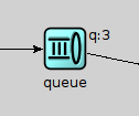

8.4.3.7 Text and Tooltip¶

It is possible to have a short text displayed next to or above the module icon or shape using the t tag. The tag lets one specify the placement (left, right, above) and the color of the text. To display text in a tooltip, use the tt tag.

The following example displays text above the module icon, and also adds tooltip text that can be seen by hovering over the module icon with the mouse.

@display("t=Packets sent: 18;tt=Additional tooltip information");

NOTE

t

tt

setTagArg()

cDisplayString

getDisplayString().setTagArg("t", 0, str);

For a detailed descripton of the display string tags, check Appendix [24].

8.4.4 Background Tags¶

The following tags of the module display string are in effect when the module itself is opened in a GUI. These tags mostly deal with the visual properties of the background rectangle.

bgb -- size, color and border of the background rectangle
bgi -- background image and its display mode
bgtt -- tooltip above the background
bgg -- background grid: color, spacing, etc.
bgu -- measurement unit of coordinates/distances

In the following example, the background area is defined to be 6000x4500 units, and the map of Europe is used as a background, stretched to fill the whole area. A grid is also drawn, with 1000 units between major ticks, and 2 minor ticks per major tick.

network EuropePlayground {     @display("bgb=6000,4500;bgi=maps/europe,s;bgg=1000,2,grey95;bgu=km");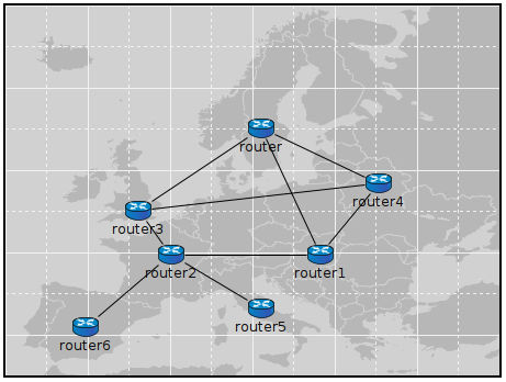

Figure: Background image and grid

The bgu tag deserves special attention. It does not affect the visual appearance, but instead it is a hint for model code on how to interpret coordinates and distances in this compound module. The above example specifies bgu=km, which means that if the model attaches physical meaning to coordinates and distances, then those numbers should be interpreted as kilometers.

More detailed information, such as what each tag argument means, is available in Appendix [24].

8.4.5 Connection Display Strings¶

Connections may also have display strings. Connections inherit the display string property from their channel types, in the same way as submodules inherit theirs from module types. The default display strings are empty.

Connections support the following tags:

ls -- line style and color
t -- text
tt -- tooltip
m -- orientation and positioning

Example of a thick, red connection:

source1.out --> { @display("ls=red,3"); } --> queue1.in++;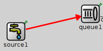

NOTE

"ls=,0"

More detailed information, such as what each tag argument means, is available in Appendix [24].

8.4.6 Message Display Strings¶

Message display strings affect how messages are shown during animation. By default, they are displayed as a small filled circle, in one of 8 basic colors (the color is determined as message kind modulo 8), and with the message class and/or name displayed under it. The latter is configurable in the Options dialog of Tkenv and Qtenv, and message kind dependent coloring can also be turned off there.

8.4.6.1 How to Specify¶

Message objects do not store a display string by default. Instead, cMessage defines a virtual getDisplayString() method that one can override in subclasses to return an arbitrary string. The following example adds a display string to a new message class:

class Job : public cMessage {   public:     const char *getDisplayString() const {return "i=msg/packet;is=vs";}     //... };

Since message classes are often defined in msg files (see chapter [6]), it is often convenient to let the message compiler generate the getDisplayString() method. To achieve that, add a string field named displayString with an initializer to the message definition. The message compiler will generate setDisplayString() and getDisplayString() methods into the new class, and also set the initial value in the constructor.

An example message file:

message Job {     string displayString = "i=msg/package_s,kind";     //... }

8.4.6.2 Tags¶

The following tags can be used in message display strings:

b -- shape, color
i -- icon
is -- icon size

NOTE

kind

message kind

The following example displays a small red box icon:

@display("i=msg/box,red;is=s");

The next one displays a 15x15 rectangle, with while fill, and with a border color dependent on the message kind:

@display("b=15,15,rect,white,kind,5");

More detailed information, such as what each tag argument means, is available in Appendix [24].

8.4.7 Parameter Substitution¶

Parameters of the module or channel containing the display string can be substituted into the display string with the $parameterName notation:

Example:

simple MobileNode {     parameters:         double xpos;         double ypos;         string fillColor;         // get the values from the module parameters xpos,ypos,fillcolor         @display("p=$xpos,$ypos;b=60,10,rect,$fillColor,black,2"); }

8.4.8 Colors¶

8.4.8.1 Color Names¶

A color may be given in several forms. One is English names: blue, lightgrey, wheat, etc.; the list includes all standard SVG color names.

Another acceptable form is the HTML RGB syntax: #rgb or #rrggbb, where r,g,b are hex digits.

It is also possible to specify colors in HSB (hue-saturation-brightness) as @hhssbb (with h, s, b being hex digits). HSB makes it easier to scale colors e.g. from white to bright red.

One can produce a transparent background by specifying a hyphen ("-") as background color.

In message display strings, kind can also be used as a special color name. It will map message kind to a color. (See the getKind() method of cMessage.)

8.4.8.2 Icon Colorization¶

The "i=" display string tag allows for colorization of icons. It accepts a target color and a percentage as the degree of colorization. Percentage has no effect if the target color is missing. Brightness of the icon is also affected -- to keep the original brightness, specify a color with about 50% brightness (e.g. #808080 mid-grey, #008000 mid-green).

Examples:

"i=device/server,gold" creates a gold server icon
"i=misc/globe,#808080,100" makes the icon greyscale
"i=block/queue,white,100" yields a "burnt-in" black-and-white icon

Colorization works with both submodule and message icons.

8.4.9 Icons¶

8.4.9.1 The Image Path¶

In the current OMNeT++ version, module icons are PNG or GIF files. The icons shipped with OMNeT++ are in the images/ subdirectory. The IDE, Tkenv and Qtenv all need the exact location of this directory to be able to load the icons.

Icons are loaded from all directories in the image path, a semicolon-separated list of directories. The default image path is compiled into Tkenv and Qtenv with the value "<omnetpp>/images;./images". This works fine (unless the OMNeT++ installation is moved), and the ./images part also allows icons to be loaded from the images/ subdirectory of the current directory. As users typically run simulation models from the model's directory, this practically means that custom icons placed in the images/ subdirectory of the model's directory are automatically loaded.

The compiled-in image path can be overridden with the OMNETPP_IMAGE_PATH environment variable. The way of setting environment variables is system specific: in Unix, if one is using the bash shell, adding a line

export OMNETPP_IMAGE_PATH="$HOME/omnetpp/images;./images"

to ~/.bashrc or ~/.bash_profile will do; on Windows, environment variables can be set via the My Computer --> Properties dialog.

One can extend the image path from omnetpp.ini with the image-path option, which is prepended to the environment variable's value.

[General] image-path = "/home/you/model-framework/images;/home/you/extra-images"

8.4.9.2 Categorized Icons¶

Icons are organized into several categories, represented by folders. These categories include:

abstract/ - symbolic icons for various devices
background/ - images useful as background, such as terrain map
block/ - icons for subcomponents (queues, protocols, etc).
device/ - network device icons: servers, hosts, routers, etc.
misc/ - node, subnet, cloud, building, town, city, etc.
msg/ - icons that can be used for messages
status/ - status icons such as up, down, busy, etc.

Icon names to be used with the i, bgi and other tags should contain the subfolder (category) name but not the file extension. For example, /opt/omnetpp/images/block/sink.png should be referred to as block/sink.

8.4.9.3 Icon Size¶

Icons come in various sizes: normal, large, small, very small, very large. Sizes are encoded into the icon name's suffix: _vl, _l, _s, _vs. In display strings, one can either use the suffix ("i=device/router_l"), or the "is" (icon size) display string tag ("i=device/router;is=l"), but not both at the same time (we recommend using the is tag.)

8.4.10 Layouting¶

OMNeT++ implements an automatic layouting feature, using a variation of the Spring Embedder algorithm. Modules which have not been assigned explicit positions via the "p=" tag will be automatically placed by the algorithm.

Spring Embedder is a graph layouting algorithm based on a physical model. Graph nodes (modules) repel each other like electric charges of the same sign, and connections act as springs that pull nodes together. There is also friction built in, in order to prevent oscillation of the nodes. The layouting algorithm simulates this physical system until it reaches equilibrium (or times out). The physical rules above have been slightly tweaked to achieve better results.

The algorithm doesn't move any module which has fixed coordinates. Modules that are part of a predefined arrangement (row, matrix, ring, etc., defined via the 3rd and further args of the "p=" tag) will be moved together, to preserve their relative positions.

NOTE

doesn't care

Caveats:

If the full graph is too big after layouting, it is scaled back so that it fits on the screen, unless it contains any fixed-position module. (For obvious reasons: if there is a module with manually specified position, we don't want to move that one). To prevent rescaling, one can specify a sufficiently large bounding box in the background display string, e.g. "b=2000,3000".
Submodule size is ignored by the present layouter, so modules with elongated shapes may not be placed ideally.
The algorithm may produce erratic results, especially for small graphs when the number of submodules is small, or when using predefined (matrix, row, ring, etc) layouts. The Relayout toolbar button can then be very useful. Larger networks usually produce satisfactory results.
The algorithm starts by placing the nodes randomly, and this initial arrangement greatly affects the end result. The algorithm has its own RNG that starts from a default seed. The Relayout button changes this seed, and this seed is persistently stored so later runs of the model will produce the same layout.

8.4.11 Changing Display Strings at Runtime¶

It is often useful to manipulate the display string at runtime. Changing colors, icon, or text may convey status change, and changing a module's position is useful when simulating mobile networks.

Display strings are stored in cDisplayString objects inside channels, modules and gates. cDisplayString also lets one manipulate the string.

As far as cDisplayString is concerned, a display string (e.g. "p=100,125;i=cloud") is a string that consist of several tags separated by semicolons, and each tag has a name and after an equal sign, zero or more arguments separated by commas.

The class facilitates tasks such as finding out what tags a display string has, adding new tags, adding arguments to existing tags, removing tags or replacing arguments. The internal storage method allows very fast operation; it will generally be faster than direct string manipulation. The class doesn't try to interpret the display string in any way, nor does it know the meaning of the different tags; it merely parses the string as data elements separated by semicolons, equal signs and commas.

To get a pointer to a cDisplayString object, one can call the components's getDisplayString() method.

NOTE

The display string can be overwritten using the parse() method. Tag arguments can be set with setTagArg(), and tags removed with removeTag().

The following example sets a module's position, icon and status icon in one step:

cDisplayString& dispStr = getDisplayString(); dispStr.parse("p=40,20;i=device/cellphone;i2=status/disconnect");

Setting an outgoing connection's color to red:

cDisplayString& connDispStr = gate("out")->getDisplayString(); connDispStr.parse("ls=red");

Setting module background and grid with background display string tags:

cDisplayString& parentDispStr = getParentModule()->getDisplayString(); parentDispStr.parse("bgi=maps/europe;bgg=100,2");

The following example updates a display string so that it contains the p=40,20 and i=device/cellphone tags:

dispStr.setTagArg("p", 0, 40); dispStr.setTagArg("p", 1, 20); dispStr.setTagArg("i", 0, "device/cellphone");

8.5 Bubbles¶

Modules can display a transient bubble with a short message (e.g. "Going down" or "Connection estalished") by calling the bubble() method of cComponent. The method takes the string to be displayed as a const char * pointer.

An example:

bubble("Going down!");

If the module often displays bubbles, it is recommended to make the corresponding code conditional on hasGUI(). The hasGUI() method returns false if the simulation is running under Cmdenv.

if (hasGUI()) {     char text[32];     sprintf(text, "Collision! (%s frames)", numCollidingFrames);     bubble(text); }

8.6 The Canvas¶

8.6.1 Overview¶

The canvas is the 2D drawing API of OMNeT++. Using the canvas, one can display lines, curves, polygons, images, text items and their combinations, using colors, transparency, geometric transformations, antialiasing and more. Drawings created with the canvas API can be viewed when the simulation is run under a graphical user interface (Tkenv or Qtenv).

Use cases for the canvas API include displaying textual annotations, status information, live statistics in the form of plots, charts, gauges, counters, etc. Other types of simulations may call for different types of graphical presentation. For example, in mobile and wireless simulations, the canvas API can be used to draw the scene including a background (like a street map or floor plan), mobile objects (vehicles, people), obstacles (trees, buildings, hills), antennas with orientation, and also extra information like connectivity graph, movement trails, individual transmissions and so on.

An arbitrary number of drawings (canvases) can be created, and every module already has one by default. A module's default canvas is the one on which the module's submodules and internal connections are also displayed, so the canvas API can be used to enrich the default, display string based presentation of a compound module.

OMNeT++ calls the items that appear on a canvas figures. The corresponding C++ types are cCanvas and cFigure. In fact, cFigure is an abstract base class, and different kinds of figures are represented by various subclasses of cFigure.

Figures can be declared statically in NED files using @figure properties, and can also be accessed, created and manipulated programmatically at runtime.

8.6.2 Creating, Accessing and Viewing Canvases¶

A canvas is represented by the cCanvas C++ class. A module's default canvas can be accessed with the getCanvas() method of cModule. For example, a toplevel submodule can get hold of the network's canvas with the following line:

cCanvas *canvas = getParentModule()->getCanvas();

Using the canvas pointer, it is possible to check what figures it contains, add new figures, manipulate existing ones, and so on.

New canvases can be created by simply creating new cCanvas objects, like so:

cCanvas *canvas = new cCanvas("liveStatistics"); // arbitrary name string

To view the contents of these additional canvases in Tkenv or Qtenv, one needs to navigate to the canvas' owner object (which will usually be the module that created the canvas), view the list of objects it contains, and double-click the canvas in the list. Giving meaningful names to extra canvas objects like in the example above can simplify the process of locating them in the Tkenv/Qtenv GUI.

8.6.3 Figure Classes¶

The base class of all figure classes is cFigure. The class hierarchy is shown in figure below.

Figure: cFigure class hierarchy

In subsequent sections, we'll first describe features that are common to all figures, then we'll briefly cover each figure class. Finally, we'll look into how one can define new figure types.

NOTE

8.6.4 The Figure Tree¶

Figures on a canvas are organized into a tree. The canvas has a (hidden) root figure, and all toplevel figures are children of the root figure. Any figure may contain child figures, not only dedicated ones like cGroupFigure.

Every figure also has a name string, inherited from cNamedObject. Since figures are in a tree, every figure also has a hierarchical name. It consists of the names of figures in the path from the root figure down to the the figure, joined with dots. (The name of the root figure itself is omitted.)

Child figures can be added to a figure with the addFigure() method, or inserted into the child list of a figure relative to a sibling with the insertBefore() / insertAfter() methods. addFigure() has two flavours: one for appending, and one for inserting at a numeric position. Child figures can be accessed by name (getFigure(name)), or enumerated by index in the child list (getFigure(k), getNumFigures()). One can obtain the index of a child figure using findFigure(). The removeFromParent() method can be used to remove a figure from its parent.

For convenience, cCanvas also has addFigure(), getFigure(), getNumFigures() and other methods for managing toplevel figures without the need to go via the root figure.

The following code enumerates the children of a figure named "group1":

cFigure *parent = canvas->getFigure("group1"); ASSERT(parent != nullptr); for (int i = 0; i < parent->getNumFigures(); i++)     EV << parent->getFigure(i)->getName() << endl;

It is also possible to locate a figure by its hierarchical name (getFigureByPath()), and to find figure by its (non-hierarchical) name anywhere in a figure subtree (findFigureRecursively()).

The dup() method of figure classes only duplicates the very figure on which it was called. (The duplicate will not have ay children.) To clone a figure including children, use the dupTree() method.

8.6.5 Creating and Manipulating Figures from NED and C++¶

As mentioned earlier, figures can be defined in the NED file, so they don't always need to be created programmatically. This possibility is useful for creating static backgrounds or statically defining placeholders for dinamically displayed items, among others. Figures defined from NED can be accessed and manipulated from C++ code in the same way as dynamically created ones.

Figures are defined in NED by adding @figure properties to a module definition. The hierarchical name of the figure goes into the property index, that is, in square brackets right after @figure. The parent of the figure must already exist, that is, when defining foo.bar.baz, both foo and foo.bar must have already been defined (in NED).

Type and various attributes of the figure go into property body, as key-valuelist pairs. type=line creates a cLineFigure, type=rectangle creates a cRectangleFigure, type=text creates a cTextFigure, and so on; the list of accepted types is given in appendix [25]. Further attributes largely correspond to getters and setters of the C++ class denoted by the type attribute.

The following example creates a green rectangle and the text "placeholder" in it in NED, and the subsequent C++ code changes the same text to "Hello World!".

NED part:

module Foo {     @display("bgb=800,500");     @figure[box](type=rectangle; coords=10,50; size=200,100; fillColor=green);     @figure[box.label](type=text; coords=20,80; text=placeholder); }

And the C++ part:

// we assume this code runs in a submodule of the above "Foo" module cCanvas *canvas = getParentModule()->getCanvas();  // obtain the figure pointer by hierarchical name, and change the text: cFigure *figure = canvas->getFigureByPath("box.label") cTextFigure *textFigure = check_and_cast<cTextFigure *>(figure); textFigure->setText("Hello World!");

8.6.6 Stacking Order¶

The stacking order (a.k.a. Z-order) of figures is jointly determined by the child order and the cFigure attribute called Z-index, with the latter taking priority. Z-index is not used directly, but an effective Z-index is computed instead, as the sum of the Z-index values of the figure and all its ancestors up to the root figure.

A figure with a larger effective Z-index will be displayed above figures with smaller effective Z-indices, regardless of their positions in the figure tree. Among figures whose effective Z-indices are equal, child order determines the stacking order. If two such figures are siblings, the one that occurs later in the child list will be drawn above the other. For figures that are not siblings, the child order within the first common ancestor matters. There are several methods for managing stacking order: setZIndex(), getZIndex(), getEffectiveZIndex(), insertAbove(), insertBelow(), isAbove(), isBelow(), raiseAbove(), lowerBelow(), raiseToTop(), lowerToBottom().

8.6.7 Transforms¶

One of the most powerful features of the Canvas API is being able to assign geometric transformations to figures. OMNeT++ uses 2D homogeneous transformation matrices, which are able to express affine transforms such as translation, scaling, rotation and skew (shearing). The transformation matrix used by OMNeT++ has the following format:

In a nutshell, given a point with its (x, y) coodinates, one can obtain the transformed version of it by multiplying the transformation matrix by the (x \ y \ 1) column vector (a.k.a. homogeneous coordinates), and dropping the third component:

The result is the point (ax+cy+t₁, bx+dy+t₂). As one can deduce, a, b, c, d are responsible for rotation, scaling and skew, and t₁ and t₂ for translation. Also, transforming a point by matrix T₁ and then by T₂ is equivalent to transforming the point by the matrix T₂ T₁ due to the associativity of matrix multiplication.

8.6.7.1 The Transform Class¶

Transformation matrices are represented in OMNeT++ by the cFigure::Transform class.

A cFigure::Transform transformation matrix can be initialized in several ways. First, it is possible to assign its a, b, c, d, t1, t2 members directly (they are public), or via a six-argument constructor. However, it is usually more convenient to start from the identity transform (as created by the default constructor), and invoke one or more of its several scale(), rotate(), skewx(), skewy() and translate() member functions. They update the matrix to (also) perform the given operation (scaling, rotation, skewing or translation), as if left-multiplied by a temporary matrix that corresponds to the operation.

The multiply() method allows one to combine transformations: t1.multiply(t2) sets t1 to the product t2*t1.

To transform a point (represented by the class cFigure::Point), one can use the applyTo() method of Transform. The following code fragment should clarify this:

// allow Transform and Point to be referenced without the cFigure:: prefix typedef cFigure::Transform Transform; typedef cFigure::Point Point;  // create a matrix that scales by 2, rotates by 45 degrees, and translates by (100,0) Transform t = Transform().scale(2.0).rotate(M_PI/4).translate(100,0);  // apply the transform to the point (10, 20) Point p(10, 20); Point p2 = t.applyTo(p);

8.6.7.2 Figure Transforms¶

Every figure has an associated transformation matrix, which affects how the figure and its figure subtree are displayed. In other words, the way a figure displayed is affected by its own transformation matrix and the transformation matrices of all of its ancestors, up to the root figure of the canvas. The effective transform will be the product of those transformation matrices.

A figure's transformation matrix is directly accessible via cFigure's getTransform(), setTransform() member functions. For convenience, cFigure also has several scale(), rotate(), skewx(), skewy() and translate() member functions, which directly operate on the internal transformation matrix.

Some figures have visual aspects that are not, or only optionally affected by the transform. For example, the size and orientation of the text displayed by cLabelFigure, in contrast to that of cTextFigure, is unaffected by transforms (and of manual zoom as well). Only the position is transformed.

8.6.7.3 Transform vs move()¶

In addition to the translate(), scale(), rotate(), etc. functions that update the figure's transformation matrix, figures also have a move() method. move(), like translate(), also moves the figure by a dx, dy offset. However, move() works by changing the figure's coordinates, and not by changing the transformation matrix.

Since every figure class stores and interprets its position differently, move() is defined for each figure class independently. For example, cPolylineFigure's move() changes the coordinates of each point.

move() is recursive, that is, it not only moves the figure on which it was called, but also its children. There is also a non-recursive variant, called moveLocal().

8.6.8 Showing/Hiding Figures¶

8.6.8.1 Visibility Flag¶

Figures have a visibility flag that controls whether the figure is displayed. Hiding a figure via the flag will hide the whole figure subtree, not just the figure itself. The flag can be accessed via the isVisible(), setVisible() member functions of cFigure.

8.6.8.2 Tags¶

Figures can also be assigned a number of textual tags. Tags do not directly affect rendering, but graphical user interfaces that display canvas content, namely Tkenv and Qtenv, offer functionality to interactively show/hide figures based on tags they contain. This GUI figure filter allows one to express conditions like "Show only figures that have tag foo or bar, but among them, hide those that also contain tag baz". Tag-based filtering and the visibility flag are in AND relationship -- figures hidden via setVisible(false) cannot be displayed using tags. Also when a figure is hidden using the tag filter, its figure subtree will also be hidden.

The tag list of a figure can be accessed with the getTags() and setTags() cFigure methods. They return/accept a single string that contains the tags separated by spaces (a tag itself cannot contain a space.)

Tags functionality, when used carefully, allows one to define "layers" that can be turned on/off from Tkenv/Qtenv.

8.6.9 Figure Tooltip, Associated Object¶

8.6.9.1 Tooltip¶

Figures may be assigned a tooltip text using the setTooltip() method. The tooltip is shown in the runtime GUI when one hovers with the mouse over the figure.

8.6.9.2 Associated Object¶

In the visualization of many simulations, some figures correspond to certain objects in the simulation model. For example, a truck image may correspond to a module that represents the mobile node in the simulation. Or, an inflating disc that represents a wireless signal may correspond to a message (cMessage) in the simulation.

One can set the associated object on a figure using the setAssociatedObject() method. The GUI can use this information provide a shortcut access to the associated object, for example select the object in an inspector when the user clicks the figure, or display the object's tooltip over the figure if it does not have its own.

CAUTION

setAssociatedObject(nullptr)

8.6.10 Specifying Positions, Colors, Fonts and Other Properties¶

8.6.10.1 Points¶

Points are represented by the cFigure::Point struct:

struct Point {     double x, y;     ... };

In addition to the public x, y members and a two-argument constructor for convenient initialization, the struct provides overloaded operators (+,-,*,/) and some utility functions like translate(), distanceTo() and str().

8.6.10.2 Rectangles¶

Rectangles are represented by the cFigure::Rectangle struct:

struct Rectangle {     double x, y,     double width, height;     ... };

A rectangle is specified with the coordinates of their top-left corner, their width and height. The latter two are expected to be nonnegative. In addition to the public x, y, width, height members and a four-argument constructor for convenient initialization, the struct also has utility functions like getCenter(), getSize(), translate() and str().

8.6.10.3 Colors¶

Colors are represented by the cFigure::Color struct as 24-bit RGB colors:

struct Color {     uint8_t red, green, blue;     ... };

In addition to the public red, green, blue members and a three-argument constructor for convenient initialization, the struct also has a string-based constructor and str() function. The string form accepts various notations: HTML colors (#rrggbb), HSB colors in a similar notation (@hhssbb), and English color names (SVG and X11 color names, to be more precise.)

However, one doesn't need to use Color directly. There are also predefined constants for the basic colors (BLACK, WHITE, GREY, RED, GREEN, BLUE, YELLOW, CYAN, MAGENTA), as well as a collection of carefully chosen dark and light colors, suitable for e.g. chart drawing, in the arrays GOOD_DARK_COLORS[] and GOOD_LIGHT_COLORS[]; for convenience, the number of colors in each are in the NUM_GOOD_DARK_COLORS and NUM_GOOD_LIGHT_COLORS constants).

The following ways of specifying colors are all valid:

cFigure::BLACK; cFigure::Color("steelblue"); cFigure::Color("#3d7a8f"); cFigure::Color("@20ff80"); cFigure::GOOD_DARK_COLORS[2]; cFigure::GOOD_LIGHT_COLORS[intrand(NUM_GOOD_LIGHT_COLORS)];

8.6.10.4 Fonts¶

The requested font for text figures is represented by the cFigure::Font struct. It stores the typeface, font style and font size in one.

struct Font {     std::string typeface;     int pointSize;     uint8_t style;     ... };

The font does not need to be fully specified, there are some defaults. When typeface is set to the empty string or when pointSize is zero or a negative value, that means that the default font or the default size should be used, respectively.

The style field can be either FONT_NONE, or the binary OR of the following constants: FONT_BOLD, FONT_ITALIC, FONT_UNDERLINE.

The struct also has a three-argument constructor for convenient initialization, and an str() function that returns a human-readable text representation of the contents.

Some examples:

cFigure::Font("Arial");  // default size, normal cFigure::Font("Arial", 12);  // 12pt, normal cFigure::Font("Arial", 12, cFigure::FONT_BOLD | cFigure::FONT_ITALIC);

8.6.10.5 Other Line and Shape Properties¶

cFigure also contains a number of enums as inner types to describe various line, shape, text and image properties. Here they are:

LineStyle

Values: LINE_SOLID, LINE_DOTTED, LINE_DASHED

This enum (cFigure::LineStyle) is used by line and shape figures to determine their line/border style. The precise graphical interpretation, e.g. dash lengths for the dashed style, depends on the graphics library that the GUI was implemented with.

CapStyle

Values: CAP_BUTT, CAP_ROUND, CAP_SQUARE

This enum is used by line and path figures, and it indicates the shape to be used at the end of the lines or open subpaths.

JoinStyle

Values: JOIN_BEVEL, JOIN_ROUND, JOIN_MITER

This enum indicates the shape to be used when two line segments are joined, in line or shape figures.

FillRule

Values: FILL_EVENODD, FILL_NONZERO.

This enum determines which regions of a self-intersecting shape should be considered to be inside the shape, and thus be filled.

Arrowhead

Values: ARROW_NONE, ARROW_SIMPLE, ARROW_TRIANGLE, ARROW_BARBED.

Some figures support displaying arrowheads at one or both ends of a line. This enum determines the style of the arrowhead to be used.

Interpolation

Values: INTERPOLATION_NONE, INTERPOLATION_FAST, INTERPOLATION_BEST.

Interpolation is used for rendering an image when it is not displayed at its native resolution. This enum indicates the algorithm to be used for interpolation.

The mode none selects the "nearest neighbor" algorithm. Fast emphasizes speed, and best emphasizes quality; however, the exact choice of algorithm (bilinear, bicubic, quadratic, etc.) depends on features of the graphics library that the GUI was implemented with.

Anchor

Values: ANCHOR_CENTER, ANCHOR_N, ANCHOR_E, ANCHOR_S, ANCHOR_W, ANCHOR_NW, ANCHOR_NE, ANCHOR_SE, ANCHOR_SW; ANCHOR_BASELINE_START, ANCHOR_BASELINE_MIDDLE,
ANCHOR_BASELINE_END.

Some figures like text and image figures are placed by specifying a single point (position) plus an anchor mode, a value from this enum. The anchor mode indicates which point of the bounding box of the figure should be positioned over the specified point. For example, when using ANCHOR_N, the figure is placed so that its top-middle point falls at the specified point.

The last three, baseline constants are only used with text figures, and indicate that the start, middle or end of the text's baseline is the anchor point.

8.6.11 Primitive Figures¶

Now that we know all about figures in general, we can look into the specific figure classes provided by OMNeT++.

8.6.11.1 cAbstractLineFigure¶

cAbstractLineFigure is the common base class for various line figures, providing line color, style, width, opacity, arrowhead and other properties for them.

Line color can be set with setLineColor(), and line width with setLineWidth(). Lines can be solid, dashed, dotted, etc.; line style can be set with setLineStyle(). The default line color is black.

Lines can be partially transparent. This property can be controlled with setLineOpacity() that takes a double between 0 and 1: a zero argument means fully transparent, and one means fully opaque.

Lines can have various cap styles: butt, square, round, etc., which can be selected with setCapStyle(). Join style, which is a related property, is not part of cAbstractLineFigure but instead added to specific subclasses where it makes sense.

Lines may also be augmented with arrowheads at either or both ends. Arrowheads can be selected with setStartArrowhead() and setEndArrowhead().

Transformations such as scaling or skew do affect the width of the line as it is rendered on the canvas. Whether zooming (by the user) should also affect it can be controlled by setting a flag (setZoomLineWidth()). The default is non-zooming lines.

Specifying zero for line width is currently not allowed. To hide the line, use setVisible(false).

[It would make sense to display zero-width lines as hairlines that are always rendered as one pixel wide regardless of transforms and zoom level, but that is not possible on all platforms.]

8.6.11.2 cLineFigure¶

cLineFigure displays a single straight line segment. The endpoints of the line can be set with the setStart()/setEnd() methods. Other properties such as color and line style are inherited from cAbstractLineFigure.

An example that draws an arrow from (0,0) to (100,100):

cLineFigure *line = new cLineFigure("line"); line->setStart(cFigure::Point(0,0)); line->setEnd(cFigure::Point(100,50)); line->setLineWidth(2); line->setEndArrowhead(cFigure::ARROW_BARBED);

The result:

8.6.11.3 cArcFigure¶

cArcFigure displays an axis-aligned arc. (To display a non-axis-aligned arc, apply a transform to cArcFigure, or use cPathFigure.) The arc's geometry is determined by the bounding box of the circle or ellipse, and a start and end angle; they can be set with the setBounds(), setStartAngle() and setEndAngle() methods. Other properties such as color and line style are inherited from cAbstractLineFigure.

For angles, zero points east. Angles that go counterclockwise are positive, and those that go clockwise are negative.

NOTE

@figure

Here is an example that draws a blue arc with an arrowhead that goes counter-clockwise from 3 hours to 12 hours on the clock:

cArcFigure *arc = new cArcFigure("arc"); arc->setBounds(cFigure::Rectangle(10,10,100,100)); arc->setStartAngle(0); arc->setEndAngle(M_PI/2); arc->setLineColor(cFigure::BLUE); arc->setEndArrowhead(cFigure::ARROW_BARBED);

The result:

8.6.11.4 cPolylineFigure¶

By default, cPolylineFigure displays multiple connecting straight line segments. The class stores geometry information as a sequence of points. The line may be smoothed, so the figure can also display complex curves.

The points can be set with setPoints() that takes std::vector<Point>, or added one-by-one using addPoint(). Elements in the point list can be read and overwritten (getPoint(), setPoint()). One can also insert and remove points (insertPoint() and removePoint().

A smoothed line is drawn as a series of Bezier curves, which touch the start point of the first line segment, the end point of the last line segment, and the midpoints of intermediate line segments, while intermediate points serve as control points. Smoothing can be turned on/off using setSmooth().

Additional properties such as color and line style are inherited from cAbstractLineFigure. Line join style (which is not part of cAbstractLineFigure) can be set with setJoinStyle().

Here is an example that uses a smoothed polyline to draw a spiral:

cPolylineFigure *polyline = new cPolylineFigure("polyline"); const double C = 1.1; for (int i = 0; i < 10; i++)     polyline->addPoint(cFigure::Point(5*i*cos(C*i), 5*i*sin(C*i))); polyline->move(100, 100); polyline->setSmooth(true);

The result, with both smooth=false and smooth=true:

8.6.11.5 cAbstractShapeFigure¶

cAbstractShapeFigure is an abstract base class for various shapes, providing line and fill color, line and fill opacity, line style, line width, and other properties for them.

Both outline and fill are optional, they can be turned on and off independently with the setOutlined() and setFilled() methods. The default is outlined but unfilled shapes.

Similar to cAbstractLineFigure, line color can be set with setLineColor(), and line width with setLineWidth(). Lines can be solid, dashed, dotted, etc.; line style can be set with setLineStyle(). The default line color is black.

Fill color can be set with setFillColor(). The default fill color is blue (although it is indifferent until one calls setFilled(true)).

NOTE

setFillColor()

setFilled(true)

Shapes can be partially transparent, and opacity can be set individually for the outline and the fill, using setLineOpacity() and setFillOpacity(). These functions accept a double between 0 and 1: a zero argument means fully transparent, and one means fully opaque.

When the outline is drawn with a width larger than one pixel, it will be drawn symmetrically, i.e. approximately 50-50% of its width will fall inside and outside the shape. (This also means that the fill and a wide outline will partially overlap, but that is only apparent if the outline is also partially transparent.)

Specifying zero for line width is currently not allowed. To hide the outline, setOutlined(false) can be used.

8.6.11.6 cRectangleFigure¶

cRectangleFigure displays an axis-aligned rectangle with optionally rounded corners. As with all shape figures, drawing of both the outline and the fill are optional. Line and fill color, and several other properties are inherited from cAbstractShapeFigure.

The figure's geometry can be set with the setBounds() method that takes a cFigure::Rectangle. The radii for the rounded corners can be set independently for the x and y direction using setCornerRx() and setCornerRy(), or together with setCornerRadius().

The following example draws a rounded rectangle of size 160x100, filled with a "good dark color".

cRectangleFigure *rect = new cRectangleFigure("rect"); rect->setBounds(cFigure::Rectangle(100,100,160,100)); rect->setCornerRadius(5); rect->setFilled(true); rect->setFillColor(cFigure::GOOD_LIGHT_COLORS[0]);

The result:

8.6.11.7 cOvalFigure¶

cOvalFigure displays a circle or an axis-aligned ellipse. As with all shape figures, drawing of both the outline and the fill are optional. Line and fill color, and several other properties are inherited from cAbstractShapeFigure.

The geometry is specified with the bounding box, and it can be set with the setBounds() method that takes a cFigure::Rectangle.

The following example draws a circle of diameter 120 with a wide dotted line.

cOvalFigure *circle = new cOvalFigure("circle"); circle->setBounds(cFigure::Rectangle(100,100,120,120)); circle->setLineWidth(2); circle->setLineStyle(cFigure::LINE_DOTTED);

The result:

8.6.11.8 cRingFigure¶

cRingFigure displays a ring, with explicitly controllable inner/outer radii. The inner and outer circles (or ellipses) form the outline, and the area between them is filled. As with all shape figures, drawing of both the outline and the fill are optional. Line and fill color, and several other properties are inherited from cAbstractShapeFigure.

The geometry is determined by the bounding box that defines the outer circle, and the x and y radii of the inner oval. They can be set with the setBounds(), setInnerRx() and setInnerRy() member functions. There is also a utility method for setting both inner radii together, named setInnerRadius().

The following example draws a ring with an outer diameter of 50 and inner diameter of 20.

cRingFigure *ring = new cRingFigure("ring"); ring->setBounds(cFigure::Rectangle(100,100,50,50)); ring->setInnerRadius(10); ring->setFilled(true); ring->setFillColor(cFigure::YELLOW);

8.6.11.9 cPieSliceFigure¶

cPieSliceFigure displays a pie slice, that is, a section of an axis-aligned disc or filled ellipse. The outline of the pie slice consists of an arc and two radii. As with all shape figures, drawing of both the outline and the fill are optional.

Similar to an arc, a pie slice is determined by the bounding box of the full disc or ellipse, and a start and an end angle. They can be set with the setBounds(), setStartAngle() and setEndAngle() methods.

For angles, zero points east. Angles that go counterclockwise are positive, and those that go clockwise are negative.

NOTE

@figure

Line and fill color, and several other properties are inherited from cAbstractShapeFigure.

The following example draws pie slice that's one third of a whole pie:

cPieSliceFigure *pieslice = new cPieSliceFigure("pieslice"); pieslice->setBounds(cFigure::Rectangle(100,100,100,100)); pieslice->setStartAngle(0); pieslice->setEndAngle(2*M_PI/3); pieslice->setFilled(true); pieslice->setLineColor(cFigure::BLUE); pieslice->setFillColor(cFigure::YELLOW);

The result:

8.6.11.10 cPolygonFigure¶

cPolygonFigure displays a (closed) polygon, determined by a sequence of points. The polygon may be smoothed. A smoothed polygon is drawn as a series of cubic Bezier curves, where the curves touch the midpoints of the sides, and vertices serve as control points. Smoothing can be turned on/off using setSmooth().

As with all shape figures, drawing of both the outline and the fill are optional. The drawing of filled self-intersecting polygons is controlled by the fill rule, which defaults to even-odd (FILL_EVENODD), and can be set with setFillRule(). Line join style can be set with the setJoinStyle().

Line and fill color, and several other properties are inherited from cAbstractShapeFigure.

Here is an example of a smoothed polygon that also demonstrates the use of setPoints():

cPolygonFigure *polygon = new cPolygonFigure("polygon"); std::vector<cFigure::Point> points; points.push_back(cFigure::Point(0, 100)); points.push_back(cFigure::Point(50, 100)); points.push_back(cFigure::Point(100, 100)); points.push_back(cFigure::Point(50, 50)); polygon->setPoints(points); polygon->setLineColor(cFigure::BLUE); polygon->setLineWidth(3); polygon->setSmooth(true);

The result, with both smooth=false and smooth=true:

8.6.11.11 cPathFigure¶

cPathFigure displays a "path", a complex shape or line modeled after SVG paths. A path may consist of any number of straight line segments, Bezier curves and arcs. The path can be disjoint as well. Closed paths may be filled. The drawing of filled self-intersecting polygons is controlled by the fill rule property. Line and fill color, and several other properties are inherited from cAbstractShapeFigure.

A path, when given as a string, looks like this one that draws a triangle:

M 150 0 L 75 200 L 225 200 Z

It consists of a sequence of commands (M for moveto, L for lineto, etc.) that are each followed by numeric parameters (except Z). All commands can be expressed with lowercase letter, too. A capital letter means that the target point is given with absolute coordinates, a lowercase letter means they are given relative to the target point of the previous command.

cPathFigure can accept the path in string form (setPath()), or one can assemble the path with a series of method calls like addMoveTo(). The path can be cleared with the clearPath() method.

The commands with argument list and the corresponding add methods:

M x y: move; addMoveTo(), addMoveRel()
L x y: line; addLineTo(), addLineRel()
H x: horizontal line; addHorizontalLineTo(), addHorizontalLineRel()
V y: vertical line; addVerticalLineTo(), addVerticalLineRel()
A rx ry phi largeArc sweep x y: arc; addArcTo(), addArcRel()
Q x1 y1 x y: curve; addCurveTo(), addCurveRel()
T x y: smooth curve; addSmoothCurveTo(), addSmoothCurveRel()
C x1 y1 x2 y2 x y: cubic Bezier curve; addCubicBezierCurveTo(), addCubicBezierCurveRel()
S x1 y1 x y: smooth cubic Bezier curve; addSmoothCubicBezierCurveTo(), addSmoothCubicBezierCurveRel()
Z: close path; addClosePath()

In the parameter lists, (x,y) are the target points (substitute (dx,dy) for the lowercase, relative versions.) For the Bezier curves, x1,y1 and (x2,y2) are control points. For the arc, rx and ry are the radii of the ellipse, phi is a rotation angle in degrees for the ellipse, and largeArc and sweep are both booleans (0 or 1) that select which portion of the ellipse should be taken.

[For more details, consult the SVG specification.]

No matter how the path was created, the string form can be obtained with the getPath() method, and the parsed form with the getNumPathItems(), getPathItem(k) methods. The latter returns pointer to a cPathFigure::PathItem, which is a base class with subclasses for every item type.

Line join style, cap style (for open subpaths), and fill rule (for closed subpaths) can be set with the setJoinStyle(), setCapStyle(), setFillRule() methods.

cPathFigure has one more property, a (dx,dy) offset, which exists to simplify the implementation of the move() method. Offset causes the figure to be translated by the given amount for drawing. For other figure types, move() directly updates the coordinates, so it is effectively a wrapper for setPosition() or setBounds(). For path figures, implementing move() so that it updates every path item would be cumbersome and potentially also confusing for users. Instead, move() updates the offset. Offset can be set with setOffset(),

In the first example, the path is given as a string:

cPathFigure *path = new cPathFigure("path"); path->setPath("M 0 150 L 50 50 Q 20 120 100 150 Z"); path->setFilled(true); path->setLineColor(cFigure::BLUE); path->setFillColor(cFigure::YELLOW);

The second example creates the equivalent path programmatically.

cPathFigure *path2 = new cPathFigure("path"); path2->addMoveTo(0,150); path2->addLineTo(50,50); path2->addCurveTo(20,120,100,150); path2->addClosePath(); path2->setFilled(true); path2->setLineColor(cFigure::BLUE); path2->setFillColor(cFigure::YELLOW);

The result:

8.6.11.12 cAbstractTextFigure¶

cAbstractTextFigure is an abstract base class for figures that display (potentially multi-line) text.

The location of the text on the canvas is determined jointly by a position and an anchor. The anchor tells how to place the text relative to the positioning point. For example, if anchor is ANCHOR_CENTER then the text is centered on the point; if anchor is ANCHOR_N then the text will be drawn so that its top center point is at the positioning point. The values ANCHOR_BASELINE_START, ANCHOR_BASELINE_MIDDLE, ANCHOR_BASELINE_END refer to the beginning, middle and end of the baseline of the (first line of the) text as anchor point. The member functions to set the positioning point and the anchor are setPosition() and setAnchor(). Anchor defaults to ANCHOR_CENTER.

The font can be set with the setFont() member function that takes cFigure::Font, a class that encapsulates typeface, font style and size. Color can be set with setColor(). The displayed text can also be partially transparent. This is controlled with the setOpacity() member function that accepts an double in the [0,1] range, 0 meaning fully transparent (invisible), and 1 meaning fully opaque.

It is also possible to have a partially transparent "halo" displayed around the text. The halo improves readability when the text is displayed over a background that has a similar color as the text, or when it overlaps with other text items. The halo can be turned on with setHalo().

8.6.11.13 cTextFigure¶

cTextFigure displays text which is affected by zooming and transformations. Font, color, position, anchoring and other properties are inherited from cAbstractTextFigure.

The following example displays a text in dark blue 12-point bold Arial font.

cTextFigure *text = new cTextFigure("text"); text->setText("This is some text."); text->setPosition(cFigure::Point(100,100)); text->setAnchor(cFigure::ANCHOR_BASELINE_MIDDLE); text->setColor(cFigure::Color("#000040")); text->setFont(cFigure::Font("Arial", 12, cFigure::FONT_BOLD));

The result:

8.6.11.14 cLabelFigure¶

cLabelFigure displays text which is unaffected by zooming or transformations, except its position. Font, color, position, anchoring and other properties are inherited from cAbstractTextFigure. The angle of the label can be set with the setAngle() method. Zero angle means horizontal (unrotated) text. Positive values rotate counterclockwise, while negative values rotate clockwise.

NOTE

@figure

The following example displays a label in Courier New with the default size, slightly transparent.

cLabelFigure *label = new cLabelFigure("label"); label->setText("This is a label."); label->setPosition(cFigure::Point(100,100)); label->setAnchor(cFigure::ANCHOR_NW); label->setFont(cFigure::Font("Courier New")); label->setOpacity(0.9);

The result:

8.6.11.15 cAbstractImageFigure¶

cAbstractImageFigure is an abstract base class for image figures.

The location of the image on the canvas is determined jointly by a position and an anchor. The anchor tells how to place the image relative to the positioning point. For example, if anchor is ANCHOR_CENTER then the image is centered on the point; if anchor is ANCHOR_N then the image will be drawn so that its top center point is at the positioning point. The member functions to set the positioning point and the anchor are setPosition() and setAnchor(). Anchor defaults to ANCHOR_CENTER.

By default, the figure's width/height will be taken from the image's dimensions in pixels. This can be overridden with thesetWidth() / setHeight() methods, causing the image to be scaled. setWidth(0) / setHeight(0) reset the default (automatic) width and height.

One can choose from several interpolation modes that control how the image is rendered when it is not drawn in its natural size. Interpolation mode can be set with setInterpolation(), and defaults to INTERPOLATION_FAST.

Images can be tinted; this feature is controlled by a tint color and a tint amount, a [0,1] real number. They can be set with the setTintColor() and setTintAmount() methods, respectively.

Images may also be rendered as partially transparent, which is controlled by the opacity property, a [0,1] real number. Opacity can be set with the setOpacity() method. The rendering process will combine this property with the transparency information contained within the image, i.e. the alpha channel.

8.6.11.16 cImageFigure¶

cImageFigure displays an image, typically an icon or a background image, loaded from the OMNeT++ image path. Positioning and other properties are inherited from cAbstractImageFigure. Unlike cIconFigure, cImageFigure fully obeys transforms and zoom.

The following example displays a map:

cImageFigure *image = new cImageFigure("map"); image->setPosition(cFigure::Point(0,0)); image->setAnchor(cFigure::ANCHOR_NW); image->setImageName("maps/europe"); image->setWidth(600); image->setHeight(500);

8.6.11.17 cIconFigure¶

cIconFigure displays a non-zooming image, loaded from the OMNeT++ image path. Positioning and other properties are inherited from cAbstractImageFigure.

cIconFigure is not affected by transforms or zoom, except its position. (It can still be resized, though, via setWidth() / setHeight().)

The following example displays an icon similar to the way the "i=block/sink,gold,30" display string tag would, and makes it slightly transparent:

cIconFigure *icon = new cIconFigure("icon"); icon->setPosition(cFigure::Point(100,100)); icon->setImageName("block/sink"); icon->setTintColor(cFigure::Color("gold")); icon->setTintAmount(0.6); icon->setOpacity(0.8);

The result:

8.6.11.18 cPixmapFigure¶

cPixmapFigure displays a user-defined raster image. A pixmap figure may be used to display e.g. a heat map. Support for scaling and various interpolation modes are useful here. Positioning and other properties are inherited from cAbstractImageFigure.

A pixmap itself is represented by the cFigure::Pixmap class.

cFigure::Pixmap stores a rectangular array of 32-bit RGBA pixels, and allows pixels to be manipulated directly. The size ($width x height$) as well as the default fill can be specified in the constructor. The pixmap can be resized (i.e. pixels added/removed at the right and/or bottom) using setSize(), and it can be filled with a color using fill(). Pixels can be directly accessed with pixel(x,y).

A pixel is returned as type cFigure::RGBA, which is a convenience struct that, in addition to having the four public uint8_t fields (red, green, blue, alpha), is augmented with several utility methods.

Many Pixmap and RGBA methods accept or return cFigure::Color and opacity, converting between them and RGBA. (Opacity is a [0,1] real number that is mapped to the 0..255 alpha channel. 0 means fully transparent, and 1 means fully opaque.)

One can set up and manipulate the image that cPixmapFigure displays in two ways. First, one can create and fill a cFigure::Pixmap separately, and set it on cPixmapFigure using setPixmap(). This will overwrite the figure's internal pixmap instance that it displays. The second way is to utilize cPixmapFigure's methods such as setPixmapSize(), fill(), setPixel(), setPixelColor(), setPixelOpacity(), etc. that delegate to the internal pixmap instance.

The following example displays a small heat map by manipulating the transparency of the pixels. The 9-by-9 pixel image is stretched to 100 units each direction on the screen.

cPixmapFigure *pixmapFigure = new cPixmapFigure("pixmap"); pixmapFigure->setPosition(cFigure::Point(100,100)); pixmapFigure->setSize(100, 100); pixmapFigure->setPixmapSize(9, 9, cFigure::BLUE, 1); for (int y = 0; y < pixmapFigure->getPixmapHeight(); y++) {     for (int x = 0; x < pixmapFigure->getPixmapWidth(); x++) {         double opacity = 1 - sqrt((x-4)*(x-4) + (y-4)*(y-4))/4;         if (opacity < 0) opacity = 0;         pixmapFigure->setPixelOpacity(x, y, opacity);     } } pixmapFigure->setInterpolation(cFigure::INTERPOLATION_FAST);

The result, both with interpolation=NONE and interpolation=FAST:

8.6.11.19 cGroupFigure¶

cGroupFigure is for the sole purpose of grouping its children. It has no visual appearance. The usefulness of a group figure comes from the fact that elements of a group can be hidden / shown together, and also transformations are inherited from parent to child, thus, children of a group can be moved, scaled, rotated, etc. together by updating the group's transformation matrix.

The following example creates a group with two subfigures, then moves and rotates them as one unit.

cGroupFigure *group = new cGroupFigure("group");  cRectangleFigure *rect = new cRectangleFigure("rect"); rect->setBounds(cFigure::Rectangle(-50,0,100,40)); rect->setCornerRadius(5); rect->setFilled(true); rect->setFillColor(cFigure::YELLOW);  cLineFigure *line = new cLineFigure("line"); line->setStart(cFigure::Point(-80,50)); line->setEnd(cFigure::Point(80,50)); line->setLineWidth(3);  group->addFigure(rect); group->addFigure(line); group->translate(100, 100); group->rotate(M_PI/6, 100, 100);

The result:

8.6.11.20 cPanelFigure¶

cPanelFigure is similar to cGroupFigure in that it is also intended for grouping its children and has no visual appearance of its own. However, it has a special behavior regarding transformations and especially zooming.

cPanelFigure sets up an axis-aligned, unscaled coordinate system for its children, canceling the effect of any transformation (scaling, rotation, etc.) inherited from ancestor figures. This allows for pixel-based positioning of children, and makes them immune to zooming.

Unlike cGroupFigure which itself has position attribute, cPanelFigure uses two points for positioning, a position and an anchor point. Position is interpreted in the coordinate system of the panel figure's parent, while the anchor point is interpreted in the coordinate system of the panel figure itself. To place the panel figure on the canvas, the panel's anchor point is mapped to position in the parent.

Setting a transformation on the panel figure itself allows for rotation, scaling, and skewing of its children. The anchor point is also affected by this transformation.

The following example demonstrates cPanelFigure behavior. It creates a normal group figure as parent for the panel, and sets up a skewed coordinate system on it. A reference image is also added to it, in order to make the effect of skew visible. The panel figure is also added to it as a child. The panel contains an image (showing the same icon as the reference image), and a border around it.

cGroupFigure *layer = new cGroupFigure("parent"); layer->skewx(-0.3);  cImageFigure *referenceImg = new cImageFigure("ref"); referenceImg->setImageName("block/broadcast"); referenceImg->setPosition(cFigure::Point(200,200)); referenceImg->setOpacity(0.3); layer->addFigure(referenceImg);  cPanelFigure *panel = new cPanelFigure("panel");  cImageFigure *img = new cImageFigure("img"); img->setImageName("block/broadcast"); img->setPosition(cFigure::Point(0,0)); panel->addFigure(img);  cRectangleFigure *border = new cRectangleFigure("border"); border->setBounds(cFigure::Rectangle(-25,-25,50,50)); border->setLineWidth(3); panel->addFigure(border);  layer->addFigure(panel); panel->setAnchorPoint(cFigure::Point(0,0)); panel->setPosition(cFigure::Point(210,200));

The screenshot shows the result at an approx. 4x zoom level. The large semi-transparent image is the reference image, the smaller one is the image within the panel figure. Note that neither the skew nor the zoom has affected the panel figure's children.

8.6.12 Compound Figures¶

Any graphics can be built using primitive (i.e. elementary) figures alone. However, when the graphical presentation of a simulation grows complex, it is often convenient to be able to group certain figures and treat them as a single unit. For example, although a bar chart can be displayed using several independent rectangle, line and text items, there are clearly benefits to being able to handle them together as a single bar chart object.

Compound figures are cFigure sublasses that are themselves composed of several figures, but can be instantiated and manipulated as a single figure. Compound figure classes can be used from C++ code like normal figures, and can also be made to be able to be instatiated from @figure properties.

Compound figure classes usually subclass from cGroupFigure. The class would typically maintain pointers to its subfigures in class members, and its methods (getters, setters, etc.) would operate on the subfigures.

To be able to use the new C++ class with @figure , it needs to be registered using the Register_Figure() macro. The macro expects two arguments: one is the type name by which the figure is known to @figure (the string to be used with the type property key), and the other is the C++ class name. For example, to be able to instantiate a class named FooFigure with @figure[...](type=foo;...), the following line needs to be added into the C++ source:

Register_Figure("foo", FooFigure);

If the figure needs to be able take values from @figure properties, the class needs to override the parse(cProperty*) method, and proably also getAllowedPropertyKeys(). We recommend that you examine the code of the figure classes built into OMNeT++ for implementation hints.

8.6.13 Self-Refreshing Figures¶

Most figures are entirely passive objects. When they need to be moved or updated during the course of the simulation, there must be an active component in the simulation that does it for them. Usually it is the refreshDisplay() method of some simple module (or modules) that contain the code that updates various properties of the figures.

However, certain figures can benefit from being able to refresh themselves during the simulation. Picture, for example, a compound figure (see previous section) that displays a line chart which is continually updated with new data as the simulation progresses. The LineChartFigure class may contain an addDataPoint(x,y) method which is called from other parts of the simulation to add new data to the chart. The question is when to update the subfigures that make up the chart: the line(s), axis ticks and labels, etc. It is clearly not very efficient to do it in every addDataPoint(x,y) call, especially when the simulation is running in Express mode when the screen is not refreshed very often. Luckily, our hypothetical LineChartFigure class can do better, and only refresh its subfigures when it matters, i.e. when the result can actually be seen in the GUI. To do that, the class needs to override cFigure's refreshDisplay() method, and place the subfigure updating code there.

Figure classes that override refreshDisplay() to refresh their own contents are called self-refreshing figures. Self-refreshing figures as a feature are available since OMNeT++ version 5.1.

refreshDisplay() is declared on cFigure as:

virtual void refreshDisplay();

The default implementation does nothing.

Like cModule's refreshDisplay(), cFigure's refreshDisplay() is invoked only under graphical user interfaces (Qtenv/Tkenv), and right before display updates. However, it is only invoked for figures on canvases that are currently displayed. This makes it possible for canvases that are never viewed to have zero refresh overhead.

Since cFigure's refreshDisplay() is only invoked when the canvas is visible, it should only be used to update local state, i.e. only local members and local subfigures. The code should certainly not access other canvases, let alone change the state of the simulation.

8.6.14 Figures with Custom Renderers¶

In rare cases it might be necessary to create figure types where the rendering is entirely custom, and not based on already existing figures. The difficulty arises from the point that figures are only data storage classes, actual drawing takes place in the GUI library such as Tkenv and Qtenv. Thus, in addition to writing the new figure class, one also needs to extend Tkenv and/or Qtenv with the corresponding rendering code. We won't go into full details on how to extend Tkenv/Qtenv here, just give you a few pointers in case you need it.

In both Tkenv and Qtenv, rendering is done with the help of figure renderer classes that have a class hierarchy roughly parallel to the cFigure inheritance tree. The base classes are incidentally called FigureRenderer. How figure renderers do their job is different in Tkenv and Qtenv: in Tkenv, rendering occurs by creating and maintaining canvas items on a Tkpath canvas; on Qtenv, they create and manipulate QGraphicsItems on a QGraphicsView. To be able to render a new figure type, one needs to create the appropriate figure renderer classes for Tkenv, Qtenv, or both.

The names of the renderer classes are provided by the figures themselves, by their getRendererClassName() methods. For example, cLineFigure's getRendererClassName() returns LineFigureRenderer. Qtenv qualifies that with its own namespace, and looks for a registered class named omnetpp::qtenv::LineFigureRenderer. If such class exists and is a Qtenv figure renderer (the appropriate dynamic_cast succeeds), an instance of that class will be used to render the figure, otherwise an error message will be issued. Tkenv does something similar.

8.7 3D Visualization¶

8.7.1 Introduction¶

OMNeT++ lets one build advanced 3D visualization for simulation models. 3D visualization is useful for wide range of simulations, including mobile wireless networks, transportation models, factory floorplan simulations and more. One can visualize terrain, roads, urban street networks, indoor environments, satellites, and more. It is possible to augment the 3D scene with various annotations. For wireless network simulations, for example, one can create a scene that, in addition to the faithful representation of the physical world, also displays the transmission range of wireless nodes, their connectivity graph and various statistics, indicates individual wireless transmissions or traffic intensity, and so on.

In OMNeT++, 3D visualization is completely distinct from display string-based and canvas-based visualization. The scene appears on a separate GUI area. Visualizing 3D scenes is currently only supported in Qtenv (i.e. it is unavailable in Tkenv.)

OMNeT++'s 3D visualization is based on the open-source OpenSceneGraph and osgEarth libraries. These libraries offer high-level functionality, such as the ability of using 3D model files directly, accessing and rendering online map and satellite imagery data sources, and so on.

8.7.1.1 OpenSceneGraph and osgEarth¶

OpenSceneGraph (openscenegraph.org), or OSG for short, is the base library. It is best to quote their web site:

"OpenSceneGraph is an open source high performance 3D graphics toolkit, used by application developers in fields such as visual simulation, games, virtual reality, scientific visualization and modeling. Written entirely in Standard C++ and OpenGL, it runs on all Windows platforms, OS X, GNU/Linux, IRIX, Solaris, HP-UX, AIX and FreeBSD operating systems. OpenSceneGraph is now well established as the world leading scene graph technology, used widely in the vis-sim, space, scientific, oil-gas, games and virtual reality industries."

In turn, osgEarth (osgearth.org) is a geospatial SDK and terrain engine built on top of OpenSceneGraph, not quite unlike Google Earth. It has many attractive features:

Able to use various street map providers, satellite imaging providers, elevation data sources, both online and offline
Data from online sources may be exported into a file suitable for offline use
Scene may be annotated with various types of graphical objects
Includes conversion between various geographical coordinate systems

In OMNeT++, osgEarth can be very useful for simulations involving maps, terrain, or satellites.

8.7.2 The OMNeT++ API for OpenSceneGraph¶

For 3D visualization, OMNeT++ basically exposes the OpenSceneGraph API. One needs to assemble an OSG scene graph in the model, and give it to OMNeT++ for display. The scene graph can be updated at runtime, and changes will be reflected in the display.

NOTE

What is a scene graph?

When a scene graph has been built by the simulation model, it needs to be given to a cOsgCanvas object to let the OMNeT++ GUI know about it. cOsgCanvas wraps a scene graph, plus hints for the GUI on how to best display the scene, for example the default camera position. In the GUI, the user can use the mouse to manipulate the camera to view the scene from various angles and distances, look at various parts of the scene, and so on.

It is important to note that the simulation model may only manipulate the scene graph, but it cannot directly access the viewer in the GUI. There is a very specific technical reason for that. The viewer may not even exist or may be displaying a different scene graph at the time the model tries to access it. The model may even be running under a non-GUI user interface (e.g. Cmdenv) where a viewer is not even part of the program. The viewer may only be influenced in the form of viewer hints in cOsgCanvas.

8.7.2.1 Creating and Accessing cOsgCanvas Objects¶

Every module has a built-in (default) cOsgCanvas, which can be accessed with the getOsgCanvas() method of cModule. For example, a toplevel submodule can get hold of the network's OSG canvas with the following line:

cOsgCanvas *osgCanvas = getParentModule()->getOsgCanvas();

Additional cOsgCanvas instances may be created simply with new:

cOsgCanvas *osgCanvas = new cOsgCanvas("scene2");

8.7.2.2 cOsgCanvas and Scene Graphs¶

Once a scene graph has been assembled, it can be set on cOsgCanvas with the setScene() method.

osg::Node *scene = ... osgCanvas->setScene(scene);

Subsequent changes in the scene graph will be automatically reflected in the visualization, there is no need to call setScene() again or otherwise let OMNeT++ know about the changes.

8.7.2.3 Viewer Hints¶

There are several hints that the 3D viewer may take into account when displaying the scene graph. Note that hints are only hints, so the viewer may choose to ignore them, and the user may also be able to override them interactively, (using the mouse, via the context menu, hotkeys or by other means).

Viewer style. The viewer style can be set with setViewerStyle() and it determines the default hints for a scene. Choices are STYLE_GENERIC that should be set for generic (non-osgEarth) scenes (default), and STYLE_EARTH for osgEarth scenes. As a rule of thumb, STYLE_EARTH should be used only when the model is loading .earth files.
Camera manipulators. The OSG viewer makes use of camera manipulators that map mouse and keyboard gestures to camera movement. Use setCameraManipulatorType() to specify a manipulator. Several camera manipulators are available: CAM_TERRAIN is suitable for flying above an object or terrain; CAM_OVERVIEW which is similar to the terrain manipulator, but does not allow rolling or looking up (one can only see the object from above); CAM_TRACKBALL that allows unrestricted movement centered around an object; and CAM_EARTH that should be used when viewing the whole Earth is useful (i.e. modeling satellites). The default setting is to choose the manipulator automatically (CAM_AUTO) based on the viewer style (CAM_OVERVIEW or CAM_EARTH).
Scene rendering. One can set the default background color for non-osgEarth scenes using setClearColor(). It is also possible to set the distances of the near and far clipping planes (setZNear() and setZFar()). Everything in the scene will be truncated to fit between these two planes. If you see parts of objects being clipped away from the scene, try to adjust these values.
Viewpoint and field of view. Default viewpoints can be set by setGenericViewpoint(cOsgCanvas::Viewpoint&) by specifying the x, y, z coordinates of the camera, the focal point and the "up" direction. For osgEarth scenarios, setEarthViewpoint(osgEarth::Viewpoint&) can be used to set the location of the observer and focal point using geographic coordinates. It is also possible to set the camera's field of view angle, with setFieldOfViewAngle().

An example code fragment that sets some viewer hints:

osgCanvas->setViewerStyle(cOsgCanvas::STYLE_GENERIC); osgCanvas->setCameraManipulatorType(cOsgCanvas::CAM_OVERVIEW); osgCanvas->setClearColor(cOsgCanvas::Color("skyblue")); osgCanvas->setGenericViewpoint(cOsgCanvas::Viewpoint(         cOsgCanvas::Vec3d(20, -30, 30), // observer         cOsgCanvas::Vec3d(30, 20, 0),   // focal point         cOsgCanvas::Vec3d(0, 0, 1)));   // UP

8.7.2.4 Making Nodes Selectable¶

If a 3D object in the scene represents a C++ object in the simulation, it would often be very convenient to be able to select that object for inspection by clicking it with the mouse.

OMNeT++ provides a wrapper node that associates its children with a particular OMNeT++ object (cObject descendant), making them selectable in the 3D viewer. The wrapper class is called cObjectOsgNode, and it subclasses from osg::Group.

auto objectNode = new cObjectOsgNode(myModule); objectNode->addChild(myNode);

NOTE

8.7.2.5 Finding Resources¶

3D visualizations often need to load external resources from disk, for example images or 3D models. By default, OSG tries to load these files from the current working directory (unless they are given with absolute path). However, loading from the folder of the current OMNeT++ module, from the folder of the ini file, or from the image path would often be more convenient. OMNeT++ contains a function for that purpose.

The resolveResourcePath() method of modules and channels accepts a file name (or relative path) as input, and looks into a number of convenient locations to find the file. The list of the search folders includes the current working directory, the folder of the main ini file, and the folder of the NED file that defined the module or channel. If the resource is found, the function returns the full path; otherwise it returns the empty string.

The function also looks into folders on the NED path and the image path, i.e. the roots of the NED and image folder trees. These search locations allow one to load files by full NED package name (but using slashes instead of dots), or access an icon with its full name (e.g. block/sink).

An example that attempts to load a car.osgb model file:

std::string fileLoc = resolveResourcePath("car.osgb"); if (fileLoc == "")     throw cRuntimeError("car.osgb not found"); auto node = osgDB::readNodeFile(fileLoc); // use the resolved path

8.7.2.6 Conditional Compilation¶

OSG and osgEarth are optional in OMNeT++, and may not be available in all installations. However, one probably wants simulation models to compile even if the particular OMNeT++ installation doesn't contain the OSG and osgEarth libraries. This can be achieved by conditional compilation.

OMNeT++ detects the OSG and osgEarth libraries and defines the WITH_OSG macro if they are present. OSG-specific code needs to be surrounded with #ifdef WITH_OSG.

An example:

... #ifdef WITH_OSG #include <osgDB/ReadFile>

Design Red Off Systemc Using Dynamic Processes

Chapters

Table of Contents

1 Introduction¶

1.1 What Is OMNeT++?¶

1.2 Organization of This Manual¶

2 Overview¶

2.1 Modeling Concepts¶

2.1.1 Hierarchical Modules¶

2.1.2 Module Types¶

2.1.3 Messages, Gates, Links¶

2.1.4 Modeling of Packet Transmissions¶

2.1.5 Parameters¶

2.1.6 Topology Description Method¶

2.2 Programming the Algorithms¶

2.3 Using OMNeT++¶

2.3.1 Building and Running Simulations¶

2.3.1.1 Running the Simulation and Analyzing the Results¶

2.3.1.2 User Interfaces¶

2.3.1.3 Component Libraries¶

2.3.1.4 Universal Standalone Simulation Programs¶

2.3.2 What Is in the Distribution¶

3 The NED Language¶

3.1 NED Overview¶

3.2 NED Quickstart¶

3.2.1 The Network¶

3.2.2 Introducing a Channel¶

3.2.3 The App, Routing, and Queue Simple Modules¶

3.2.4 The Node Compound Module¶

3.2.5 Putting It Together¶

3.3 Simple Modules¶

3.4 Compound Modules¶

3.5 Channels¶

3.6 Parameters¶

3.6.1 Assigning a Value¶

3.6.2 Expressions¶

3.6.3 volatile¶

3.6.4 Units¶

3.6.5 XML Parameters¶

3.7 Gates¶

3.8 Submodules¶

3.9 Connections¶

3.9.1 Channel Specification¶

3.9.2 Reconnecting Gates¶

3.9.3 Channel Names¶

3.10 Multiple Connections¶

3.10.1 Examples¶

3.10.1.1 Chain¶

3.10.1.2 Binary Tree¶

3.10.1.3 Random Graph¶

3.10.2 Connection Patterns¶

3.10.2.1 "Subgraph of a Full Graph"¶

3.10.2.2 "Connections of Each Node"¶

3.10.2.3 "Enumerate All Connections"¶

3.11 Parametric Submodule and Connection Types¶

3.11.1 Parametric Submodule Types¶

3.11.2 Conditional Parametric Submodules¶

3.11.3 Parametric Connection Types¶

3.12 Metadata Annotations (Properties)¶

3.12.1 Property Indices¶

3.12.2 Data Model¶

3.12.3 Overriding and Extending Property Values¶

3.13 Inheritance¶

3.14 Packages¶

3.14.1 Overview¶

3.14.2 Name Resolution, Imports¶

3.14.3 Name Resolution With "like"¶

3.14.4 The Default Package¶

4 Simple Modules¶

4.1 Simulation Concepts¶

4.1.1 Discrete Event Simulation¶

4.1.2 The Event Loop¶

4.1.3 Events and Event Execution Order in OMNeT++¶

4.1.4 Simulation Time¶

4.1.5 FES Implementation¶

4.2 Components, Simple Modules, Channels¶

4.3 Defining Simple Module Types¶

4.3.1 Overview¶

4.3.2 Constructor¶

4.3.3 Initialization and Finalization¶

4.4.1.7 Pros and Cons of Using `handleMessage()`¶

4.4.2.7 Pros and Cons of Using `activity()`¶